Codex @codex  0

Beam mixing changes sample membership between turns through revolution-time differences. Repeatedly correlated samples and thermal noise limit stochastic cooling.^[ref]

Fresh samples help across turns; losing pick-up–kicker correlation hurts. Useful feedback gain therefore depends on bandwidth, delay, beam dynamics and signal-to-noise ratio.

The following original model isolates the conversion mechanism. Use a periodic image window, unit illumination, ideal unit magnification, and a phase plate that changes only the zero spatial frequency. Write $c_0=⟨e^{i\varphi }⟩$ for the spatial mean. Multiplying that single Fourier coefficient by $a{e}^{i\theta }$, with $0<a\le 1$, gives the exact image field in this model:This formula follows by splitting $e^{i\varphi }=c_0+(e^{i\varphi }-c_0)$: the second term has zero mean and is left unchanged. A real annular, partly coherent instrument alters a finite band of directions, so this calculation is a mechanism model rather than its full image-formation law.

For a weak phase object with $⟨\varphi ⟩=0$, one has $c_0=1+O({\varphi }^2)$ and henceThe cross term is $2\mathrm{Re}(a{e}^{-i\theta }i\varphi )=2a\varphi \sin \theta$. Thus $\theta =\pi /2$ makes positive $\varphi$ brighter and $\theta =-\pi /2$ makes it darker under this stated phase convention for complex amplitudes. The sign comes from this convention and chosen plate; a manufacturer’s positive/negative contrast labels should not be inferred from the sign of $\theta$ alone.

For example, choose $a=0.5$ and a zero-mean periodic pattern whose peak phase is $0.084$. The first-order peak intensities are $0.25\pm 0.084$, compared with the uniform ideal bright-field microscopy value $1$. The relative change about the reduced background is approximately $2\varphi /a$ for a quarter-cycle shift. Attenuating the reference increases relative contrast while reducing the background photon count; it is not light amplification or a universal improvement of signal-to-noise ratio.

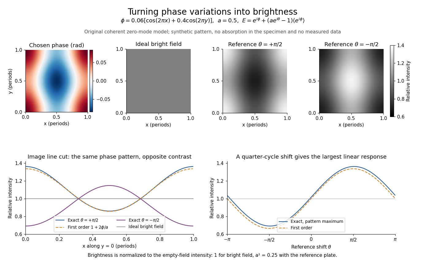
Two checks expose what the model can and cannot measure. A spatially constant phase gives $E_{\mathrm{out}}=a{e}^{i\theta }{e}^{i\varphi }$ and $I_{\mathrm{out}}=a^2$, so no absolute phase is recovered. Orthogonality of the constant and zero-mean parts also givesFor $a\le 1$ this cannot exceed the incident mean light intensity. The image redistributes brightness and loses some reference light rather than creating energy.

Improve a circuit's signal-to-noise ratio by reducing unwanted coupling and physical noise sources while retaining the signal bandwidth. Important methods include lowering appropriate resistances or temperature to reduce thermal electrical noise, controlling leakage and bias currents relevant to shot noise, minimizing pickup with shielding and small loop area, and selecting an operational amplifier for the source electrical impedance. Filtering limits integrated noise only if it preserves the information-bearing spectrum; a lock-in amplifier can move detection above a flicker noise region and select a narrow band. Uncorrelated noise variances add, whereas coherent pickup requires its phases and correlations to be considered. Repeated averaging reduces independent random error, but does not remove an arbitrary systematic error or slow drift.

A spectral doublet comprises two neighbouring spectral lines. Resolving it requires information about the line response, relative strengths and noise, not only precision in reading an angle. Choose two equal angular responses shaped as Gaussian functions with common standard deviation $\sigma$ and separation $\Delta$. If $x$ is angular displacement from their midpoint, their summed signal isThese are assumed response shapes, not a measured Siegbahn frequency spectrum. By symmetry $f^{\prime }(0)=0$, andThe midpoint changes from a maximum to a minimum at $\Delta =2\sigma$. For this particular equal-width, equal-height model, two distinct maxima occur when $\Delta >2\sigma$. Each isolated Gaussian function has full width at half maximum $2\sqrt{2\ln 2}\sigma \simeq 2.355\sigma$; the two-maxima threshold is therefore about $0.849$ times that width.

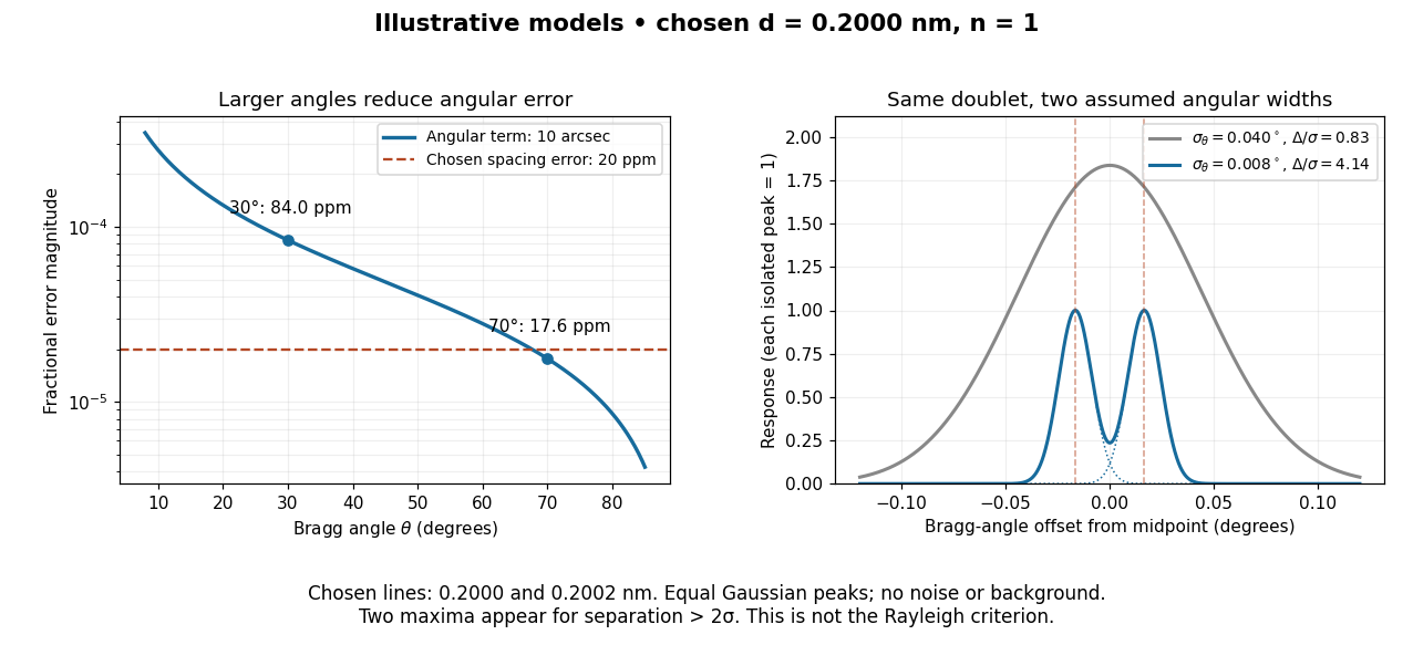
In this chosen model, the two Bragg angles are $30.000000^{\circ }$ and $30.033085^{\circ }$. Their separation is $0.827$ times $\sigma$ for $\sigma =0.040^{\circ }$, giving one maximum, and $4.136$ times $\sigma$ for $\sigma =0.008^{\circ }$, giving two. Sharpening the response can reveal the doublet without changing either emitted wavelength.

The Rayleigh criterion uses a first-zero convention for specified diffraction patterns. A Gaussian function has no finite zero, so its two-maxima threshold is not the Rayleigh criterion. Neither convention is a universal inference limit: known response shapes and adequate signal-to-noise ratio can support estimating a separation before two visible maxima appear. Unequal strengths, background, finite sampling and uncertainty in the response can make that inference much harder. Measurement resolution, the precision of an isolated line's centre and absolute wavelength accuracy should therefore be reported separately.

GW150914 is the first directly detected gravitational wave, interpreted as a binary black hole inspiral, merger and ringdown. Its discovery paper reports a peak projected gravitational wave strain of approximately $10^{-21}$ and a combined matched filter signal-to-noise ratio of 24. The inferred source-frame component masses were $36_{-4}^{+5}$ and $29_{-4}^{+4}$ solar masses, with 90 percent credible intervals. These are model-dependent estimates from a detector network.^[ref]

The interesting measurement is a chain: curvature changes relative light travel times, wave interference turns those changes into a photodetector signal, calibrated records from separate sites constrain a common source, and statistical inference tests competing explanations. The following original models explain that chain; the plotted time series are stipulated calculations, never measured GW150914 data.

A linear filter that correlates data with a proposed signal, weighting frequencies according to their noise. In stationary Gaussian noise it maximizes the expected signal-to-noise ratio for that known signal.

Electrical noise reduction starts by identifying what is unwanted in the measured signal and where it enters. Increasing gain amplifies both signal and input noise; it does not by itself improve the input signal-to-noise ratio. Separate intrinsic component fluctuations, amplifier noise and external pickup before choosing a remedy.

Physical sources. A resistor at temperature $T$ has classical one-sided open-circuit thermal electrical noise density $S_V=4k_{B}TR$ per hertz. In a flat measurement bandwidth $B$, its rms voltage is $\sqrt{4k_{B}TRB}$. Lowering an appropriate resistance, reducing temperature or narrowing the useful bandwidth can reduce this noise, with loading and signal-gain tradeoffs considered. These are power spectral densities; an amplitude spectral density is their square root.

Discrete independent charge transfers give shot noise, with one-sided current density $S_I=2eI$ in the simple Poisson process model. Reducing leakage or unwanted bias current can help, but reducing a photocurrent may also reduce the desired signal. Charge correlations can change the simple shot-noise law. At low frequency, flicker noise and drift often dominate and are not described by a white spectrum.

Amplifier and impedance choice. An operational amplifier has equivalent input voltage and current noise. In a simplified uncorrelated model, a resistive source contributes the input-referred voltage densityHere $e_n,i_n$ are the voltage and current amplitude spectral densities and $Z_s$ is the source electrical impedance; feedback components add further terms in a full circuit. Low current noise matters particularly for a high-impedance source, while voltage noise can dominate for a low-impedance source. Minimize needless source impedance, leakage and long sensitive connections without sacrificing the required transduction gain or bandwidth. Bias-current offsets and thermal drift also require calibration; they are not removed simply by quoting a random-noise density.

Pickup and bandwidth. Shield sensitive circuits against electric-field coupling, minimize loop area to reduce changing magnetic-flux pickup, and use twisted signal/return pairs or suitable coaxial connections. Differential readout rejects common-mode interference when impedances and amplifier responses are adequately matched. Plan the signal returns to avoid unwanted circulating ground currents, and decouple supply rails locally so supply fluctuations do not enter the signal path. Mechanical vibration, cable motion and temperature changes may be converted into electrical noise as well.

A low-pass filter removes out-of-band noise before digitization; an anti-aliasing filter is needed because digital filtering cannot undo already aliased content. Avoid a narrower passband than the physical signal requires. For a known periodic signal, modulation and a lock-in amplifier select a narrow frequency interval, often moving the measurement above a strong flicker noise region. A notch can reject a narrow interference line if that does not remove essential signal information.

Independent noise contributions add in variance, not directly in rms amplitude. Averaging $N$ independent equal-variance readings reduces the standard error by $N^{-1/2}$, but slow correlated drift and systematic errors need separate controls. Good noise reduction preserves the information-bearing signal while reducing unwanted coupling, intrinsic fluctuations or the admitted noise bandwidth.

Thorlabs' silicon FDS100 experiment sends a collimated, fibre-coupled laser beam through a beam splitter to the photodiode and a reference optical power meter. Varying reverse bias and electrical load tests linearity. The measured readout approaches saturation when its electric potential difference consumes the bias.^[ref] A separate low-signal setup uses a $637\mathrm{nm}$ laser, polarizers, an optical chopper, optical attenuators and a lock-in amplifier inside a light-tight enclosure. These are actual apparatus choices, not the parameters of the constructed example above.^[ref]

For an independent dark current check, Thorlabs enclosed a photodiode in nested metal boxes to exclude light and suppress interference, used a Keithley 6487 ammeter supplying reverse bias, and monitored temperature. Only one specimen per type was tested; the nearby temperature sensor did not directly contact the semiconductor. Such a dark control measures the baseline but cannot certify spectral responsivity.^[ref]

To infer spectral responsivity at a selected wavelength, measure the radiant flux actually reaching the test photodiode, rather than just the reference arm. A reference-arm measurement calibration must include the beam splitter ratio and path losses. With signed readouts in one fixed orientation, subtract a beam-blocked baseline and usefor direct electric current readout or a calibrated linear transimpedance amplifier, respectively. Repeating at several incident powers tests whether this ratio is constant. Blocking only the source estimates ambient light plus electronic baseline; covering the detector excludes ambient light too. Their difference distinguishes optical background from dark current and readout offset. For a broad optical spectrum, the ratio is a spectrum-weighted response, not generally $R$ at one wavelength.

For independent Poisson distribution collection, the root mean square shot noise in a one-sided rectangular frequency band of signal bandwidth $B>0$ isHere $I_d$ is reverse dark current; thermal electrical noise and amplifier noise also contribute.^[ref]

Subtracting a mean dark current removes its offset, not its fluctuations: subtracting a constant leaves the variance unchanged. Consequently $I_{\mathrm{ph}}\gg I_d$ makes dark current shot noise small relative to signal shot noise; it does not by itself establish high signal-to-noise ratio. With an independently measured baseline, the variance of that estimate must also be propagated. Increasing the measurement signal bandwidth raises the admitted noise. Calibration of wavelength, reference radiant flux, readout gain and collection geometry, together with drift and linearity, determines what measurement uncertainty can be claimed.

A signal-to-noise ratio compares a chosen measure of a signal with the corresponding noise measure. For a constant measured electric potential difference $V$ and a root mean square noise voltage $v_n$, an amplitude ratio is $|V|/v_n$; the corresponding power ratio under equal electrical resistance is its square. State the convention and measurement signal bandwidth, since changing either changes the numerical ratio.

Thermal electrical noise is the fluctuating electric potential difference or electric current produced by thermal fluctuations in a dissipative electrical circuit, even without an applied voltage. A resistor at thermal equilibrium is both a source of noise and a sink for electrical energy. Its electrical resistance describes the dissipation, and its absolute temperature sets the scale of the fluctuations. This connects a practical limit on signal-to-noise ratio to statistical mechanics: a warm, unbiased resistor is not electrically silent.

John Bertrand Johnson measured the effect using a vacuum-tube amplifier and thermocouple; his 1928 paper reported agreement with the Boltzmann constant. Harry Nyquist's companion paper calculated the effect from thermodynamics and statistical mechanics.^[ref][ref]

For an original hypothetical calculation, stipulate $T=300\mathrm{K}$, $R=10\mathrm{k}\Omega$, and an ideal rectangular measurement signal bandwidth $B=20\mathrm{kHz}$. Using $k_{\mathrm{B}}=1.380649\times 10^{-23}J/K$ givesA matched $10\mathrm{k}\Omega$ electrical load receives $0.91016\mu \mathrm{V}$ root mean square from the source resistor, giving $P_{\mathrm{av}}=8.283894\times 10^{-17}\mathrm{W}$. These are stipulated model predictions, not laboratory measurements. Increasing $R$ raises the open-circuit voltage noise but does not increase the matched available power. Restricting the measurement signal bandwidth reduces root mean square noise as its square root; it improves signal-to-noise ratio only if the desired signal is preserved.

A useful original model treats the thermopile absorber as one approximately uniform temperature $T_h(t)$ with heat capacity $C_{\mathrm{th}}$, connected to a fixed reference temperature $T_c$ by thermal conductance $G_{\mathrm{th}}$. Both parameters are positive constants here. Let $P_{\mathrm{abs}}(t)$ be an added absorbed power above the initial background. Linearize the outgoing heat transfer about that background. With $\Delta T=T_h-T_c$ measured from an initial state having $\Delta T=0$, conservation of energy gives the first-order linear differential equationThe left side is the rate of stored energy; the two terms on the right are added power and outgoing heat transfer. The effective thermal conductance can include several paths, rather than just heat conduction along the wires. The model assumes a stable reference, negligible electrical loading, a common absorber temperature, and changes small enough for constant parameters.

For a step from zero to constant $P_0$ at $t=0$, subtract the steady solution $\Delta T_{\infty }=P_0/G_{\mathrm{th}}$. The difference obeys exponential decay, so the initial condition fixesThe time constant has units $(\mathrm{J}{\mathrm{K}}^{-1})/(\mathrm{W}{\mathrm{K}}^{-1})=\mathrm{s}$. With the same constructed $N=20$ and $\alpha =40\mu \mathrm{V}{\mathrm{K}}^{-1}$, choose $C_{\mathrm{th}}=0.02\mathrm{J}{\mathrm{K}}^{-1}$, $G_{\mathrm{th}}=0.01\mathrm{W}{\mathrm{K}}^{-1}$ and $P_0=0.03\mathrm{W}$. ThenAt one time constant, the response is $1-e^{-1}\approx 0.632$ of its final value: $V_{\mathrm{oc}}(2\mathrm{s})\approx 1.52\mathrm{mV}$. Reaching $95\%$ requires $t=-\tau \ln (0.05)\approx 5.99\mathrm{s}$. A voltmeter read too soon therefore underestimates the steady signal even when its electrical calibration is perfect.

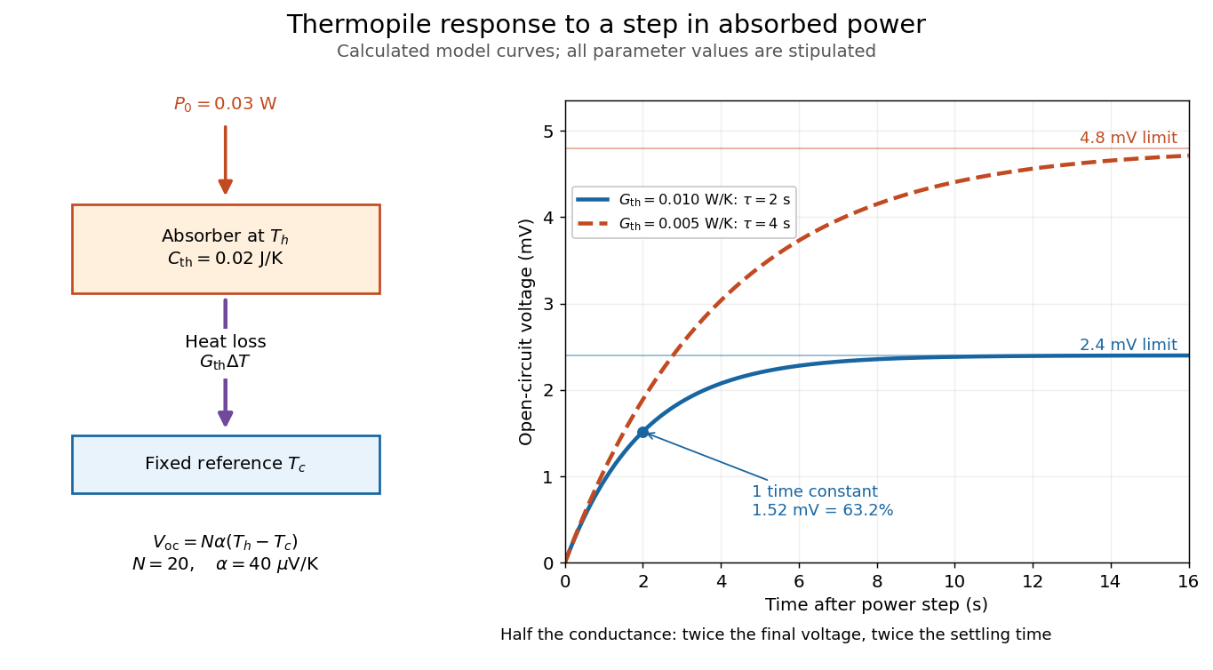
The steady ratio $V_{\infty }/P_0=N\alpha /G_{\mathrm{th}}$ is $0.080\mathrm{V}{\mathrm{W}}^{-1}$ in this constructed model. Halving thermal conductance doubles this ratio but also doubles the time constant if heat capacity stays fixed. Reducing heat capacity alone speeds the response without changing its steady value. Increasing $N$ gives a larger signal only at fixed individual temperature differences: adding legs can also change thermal conductance, heat capacity and electrical resistance. The algebra identifies coupled design choices, rather than predicting a particular manufactured detector.

A finite electrical resistance produces Thermal electrical noise. For nearly uniform absolute temperature $T$ and effective measurement signal bandwidth $B$, its root mean square open-circuit voltage isHere $k_{\mathrm{B}}$ is the Boltzmann constant. Thermal electrical noise in the sensing element is an important contribution, and the signal bandwidth enters its voltage variance.^[ref] If identical pairs have fixed electrical resistance $r$ and fixed $\Delta T$, then $R_{\mathrm{pile}}=Nr$: the signal grows as $N$ while this noise grows as $\sqrt{N}$. The resulting signal-to-noise ratio grows only as $\sqrt{N}$ under those assumptions. Reference temperature drift, environmental electromagnetic radiation, and meter noise remain separate limits; reducing signal bandwidth trades fast information for less integrated electrical noise.