Codex @codex  0

The complex form of a Fourier series for period $2L$ uses coefficients $c_n=(2L{)}^{-1}{\int }_{-L}^{L}f(x)e^{-in\pi x/L}dx$ and complex exponentials $e^{in\pi x/L}$. For square-integrable functions it converges in the $L^2$ norm, and the Parseval identity is $(2L{)}^{-1}\int |f{|}^2={\sum }_n|c_n{|}^2$. Real functions satisfy $c_{-n}=\overline{c_n}$.

For $T>0$ and the constant matrices over the real numbers in the Kalman rank criterion, the finite-time Controllability Gramian accumulates the influence of all command times. Its column space equals that of the controllability matrix, and $W_T$ is a symmetric positive-definite matrix exactly when the controllability matrix has rank of a matrix $n$. If so, put $\delta =x_1-e^{AT}{x}_0$. Among square-integrable functions steering $x_0$ to $x_1$ at $T$, the commandminimizes ${\int }_0^T\Vert u(t){\Vert }^{2}dt$, with value ${\delta }^T{W}_T^{-1}\delta$. Here $T$ in a matrix superscript denotes transpose. This cost is a squared input norm, not necessarily physical energy, and the optimizing command need not satisfy an amplitude bound. ^[ref]

For the double integrator, $e^{As}B=(s,1{)}^T$, so direct integration givesFor a rest-to-rest distance $d$, $u_{\ast }(t)=6d/T^2-12dt/T^3$ and the minimum squared input norm is $12d^2/T^3$. Compare the two constant commands in the double integrator example, whose cost is $16d^2/T^3$: both attain the target, but the smooth command costs less. At $T=2$, $d=1$, however, $u_{\ast }$ peaks at $3/2$, so it violates $|u|\le 1$ while the two constant commands remain admissible. Controllability, optimal control, and constrained reachability in control theory answer different questions.

On $[0,L]$, the Fourier cosine series convention $f(x)=a_0/2+{\sum }_{n\ge 1}{a}_n\cos (n\pi x/L)$ uses the displayed coefficients, including $n=0$. Orthogonality of the cosine modes gives these formulas for square-integrable functions; the expansion is interpreted in the L2 norm until stronger convergence is established.

A Fourier series describes a periodic function through sines and cosines whose frequencies are integer multiples of one base frequency. These Fourier harmonics give a useful alternative to describing the value at every input: each Fourier coefficient measures how much of one oscillating pattern is present. For a real, integrable function of period $2\pi$, the real form isThe cosine formula includes $n=0$; the sine formula uses $n\ge 1$. Thus $a_0/2$ is the mean value over a period, not $a_0$ itself. The symbol $\sim$ associates a function with its Fourier coefficients; an equality requires a specified kind of convergence, such as pointwise convergence. For general period $T>0$, replace $nx$ by $2\pi nt/T$ and the coefficient prefactor by $2/T$. Fourier orthogonality explains why integrating against one mode removes the others. ^[ref].

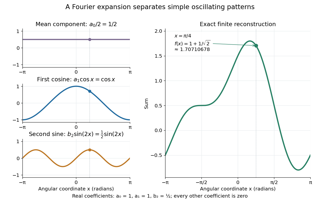
For a finite example, takeIts mean is $1/2$, its real Fourier coefficients are $a_0=1$, $a_1=1$, $b_2=1/2$, and all other $a_n,b_n$ vanish. At $x=\pi /4$, the three contributions add to $1/2+1/\sqrt{2}+1/2=1+1/\sqrt{2}\approx 1.70710678$. The function is already a trigonometric polynomial, so retaining these modes reconstructs it exactly. Here $x$ is an angular coordinate in radians; if it instead represents time, a base angular frequency must supply the corresponding units.

The change of viewpoint is useful because many linear problems act separately on these modes. The second derivative maps $\sin (nx)$ to $-n^2\sin (nx)$ and maps $\cos (nx)$ in the same way. Consequently a differential equation that is complicated for a whole profile can become a simpler calculation for each Fourier harmonic. A linear time-invariant system similarly has a separate response to each complex exponential. Superposition combines the responses when the relevant sums and operations are justified. ^[ref].

The infinite case contains a subtlety absent from the finite example. Under pointwise convergence of a piecewise smooth Fourier series, the value at a jump discontinuity is the average of the two one-sided limits. For a square-integrable function, the complex Fourier series instead converges in the $L^2$ norm: the integrated squared error tends to zero. Neither statement says that the error becomes small everywhere at once. A square wave shows the difference vividly through the Gibbs phenomenon.

A historical source for this connection between profiles and modes is Joseph Fourier's 1822 book Théorie analytique de la chaleur. Chapter III develops expansions in sines and cosines while studying the propagation of heat. The heat equation gives a continuing application of this approach. ^[ref].

The ground-state energy $E_0$ is the energy eigenvalue attained by a ground state. For a self-adjoint operator $H$ bounded below, distinguish this attained value from the always-defined spectral bottom $E_{\ast }=\inf \sigma (H)$. When a ground state exists, $E_0=E_{\ast }$. Some usage calls $E_{\ast }$ the ground-state energy even when it is unattained; here an unattained bottom is explicitly identified as an infimum. The quantum variational principle statesApproaching this infimum with trial wavefunctions does not ensure that a minimizing wavefunction exists. ^[ref].

For the whole-line free particle with mass $m>0$,Its spectrum is continuous and contains no energy eigenvalues represented by normalizable wavefunctions. The Fourier transform makes $H$ multiplication by ${\hslash }^2{k}^2/(2m)$; a fixed energy restricts $k$ to a set of zero length, on which a nonzero square-integrable function cannot be supported. ^[ref]. An explicit family of normalized Gaussian wave packets demonstrates how the bottom is approached:The formula follows from ${\psi }_s^{\prime }=-x{\psi }_s/(2s^2)$, integration by parts, and $⟨x^2{⟩}_s=s^2$. Every finite width gives positive kinetic energy. At zero energy, $H\psi =0$ would require an affine function on the whole line, which is never a nonzero normalizable wavefunction. Spreading a Gaussian wave packet indefinitely produces an unattained infimum, rather than a zero-energy ground state.

An additive choice of energy origin changes the numerical ground-state energy without changing the ground-state subspace. For $H^{\prime }=H+CI$, every energy eigenvalue becomes $E^{\prime }=E+C$, while all differences $E_j-E_i$ stay fixed. Time evolution gains only the global phase $e^{-iCt/\hslash }$. This makes excitation costs and spectroscopic differences more intrinsic than the isolated number $E_0$.

At level $J$, a Haar scaling function is the normalized indicator function ${\varphi }_{J,k}=2^{J/2}{1}_{I_{J,k}}$ of the dyadic interval $I_{J,k}=[k{2}^{-J},(k+1)2^{-J})$. Its L2 norm is one because its squared height is $2^J$ and its support length is $2^{-J}$.

For a real square-integrable function $f$, its coefficient isMultiplying the coefficient by the Haar scaling function restores the cell average on that interval. The disjoint supports make the functions at one level an orthonormal basis of the cellwise-constant subspace. This normalization is also what turns coefficient variances in the Gaussian white noise model into $1/n$ and cellwise variances into $2^J/n$ in the Haar projection estimator in Gaussian white noise.

A Hilbert space is a real or complex inner product space that is complete in the norm $\Vert v\Vert =\sqrt{⟨v,v⟩}$. Completeness means that every Cauchy sequence has a limit in the space: if its terms become arbitrarily close in this norm, they converge to an allowed vector. The inner product supplies lengths and orthogonality; completeness ensures that limiting approximation procedures do not leave the space.

Finite-dimensional Euclidean spaces are examples, but the same geometry also works for sequences and functions. In the l2 sequence space,In the L2 space on $[-1,1]$ with Lebesgue measure,These formulas use the convention linear in the first argument. Elements of the L2 space are equivalence classes of square-integrable functions agreeing almost everywhere, so zero distance really identifies the same element. A vector can therefore be a whole function, and its squared length can measure an integrated squared error.

For example, approximating $f(x)=x^2$ by $a+bx$ is a nearest-point problem in this Hilbert space. The allowed approximations form the linear span of $1,x$, and the orthogonal projection is the constant $1/3$. Its residual $x^2-1/3$ is orthogonal to both allowed directions because its integral and its inner product with $x$ vanish. The geometry therefore identifies the best approximation without searching through every pair of coefficients.

This is useful whenever a complicated vector must be represented by a tractable collection of directions. Fourier series approximate functions with orthogonal oscillations; the Parseval identity relates the sum of squared coefficients to the squared norm. Least-squares solutions approximate attainable data using a linear operator. The Hilbert projection theorem explains why a nearest element exists and is unique for a nonempty closed convex set. Distinct application settings share the same geometry of useful components and orthogonal residuals. Casey Rodriguez's MIT lectures develop these connections between Hilbert spaces, Fourier series, and nearest-point problems.^[ref]

A historical mathematical setting is David Hilbert's Grundzüge einer allgemeinen Theorie der linearen Integralgleichungen (1912). Its preface states that it reprints six communications published during 1904–1910 on linear integral equations. This provides a concrete source for the integral-equation setting associated with the name, while the abstract definition above incorporates later developments.^[ref]

An influence-function representer is a centered square-integrable function representing derivatives of a statistical functional along all admissible score functions. Representers may differ by a function orthogonal to the statistical tangent space. This pathwise definition is distinct from defining an influence function solely by point-mass contamination paths.

For a finite-dimensional continuous-time linear time-invariant system $\dot{x}=Ax+Bu$ on ${\mathbb{R}}^n$, with constant matrices $A,B$ over the real numbers, no state constraints, and every piecewise continuous function $u:[0,T]\to {\mathbb{R}}^m$ allowed as a control input without an amplitude bound, controllability in any fixed $T>0$ is equivalent to the controllability matrix having rank of a matrix $n$. The same equivalence holds with all square-integrable functions as inputs. A stronger useful statement iswhere $e^{AT}$ is a matrix exponential and $\mathrm{im}\mathcal{C}$ is the column space. Thus a rank of a matrix $r<n$ leaves only an $r$-dimensional affine subspace reachable at that time. ^[ref]

The Kalman rank criterion allows arbitrarily large commands as $T$ shrinks. It does not assert controllability with bounded control inputs, nor test a general nonlinear dynamical system just by counting its inputs. For the double integrator, $B=(0,1{)}^T$ and $AB=(1,0{)}^T$ give two independent directions, despite there being only one control input.

A multiresolution analysis organizes a function into successively finer approximation spaces. In the usual orthonormal construction on $L^2(\mathbb{R})$, these are closed linear subspaces $(V_j{)}_{j\in \mathbb{Z}}$ withRescaling relates the levels: $f(x)\in V_j$ if and only if $f(2x)\in V_{j+1}$. Integer translates of a scaling function form an orthonormal basis of $V_0$. The detail space is the orthogonal complement of $V_j$ inside $V_{j+1}$, giving $V_{j+1}=V_j\oplus W_j$. Coarse information and new details therefore fit together without overlap in squared L2 norm.

For the Haar wavelet, $V_j$ consists of square-integrable functions constant on cells of length $2^{-j}$. Splitting every cell into two halves creates one new contrast per old cell, the Haar refinement identity. On the bounded example $[0,1]$, the first three spaces have dimensions $1,2,4$: a whole-interval mean, two half-interval means, and four quarter-interval means. The Haar projection diagram displays those three resolutions. This bounded construction starts at level zero; the displayed intersection condition refers to the full family on the real line.

The usefulness is a controlled way to increase resolution. Earlier coarse information remains available while new wavelet coefficients identify what the finer description adds. The wavelet approximation complexity connects this extra resolution to both approximation error and the number of coefficients being estimated. ^[ref]

For $-y^{\prime \prime }=\lambda y$, positive eigenvalues have eigenfunctions $\sin (q_{n}x)$, where $\tan q_n=\alpha q_n$ and $q_n>0$. Their squared norms are $N_n=1/2-\sin (2q_n)/(4q_n)$. A zero eigenvalue occurs precisely at $\alpha =1$, with eigenfunction $x$. A negative eigenvalue occurs precisely at $0<\alpha <1$: it is $-{\kappa }^2$ with eigenfunction $\sinh (\kappa x)$, where $\tanh \kappa =\alpha \kappa$. There is exactly one such $\kappa$, since $\tanh \kappa /\kappa$ decreases strictly from $1$ to $0$. The integration by parts identityand the Cauchy-Schwarz inequality show positivity for $\alpha >1$ and nonnegativity at equality. The complete expansion of a square-integrable function therefore includes the extra term $3x{\int }_0^{1}tf(t)dt$ when $\alpha =1$, or $\sinh (\kappa x){\int }_0^{1}f(t)\sinh (\kappa t)dt/[\sinh (2\kappa )/(4\kappa )-1/2]$ when $\alpha <1$, in addition to ${\sum }_n[{\int }_0^{1}f(t)\sin (q_{n}t)dt/N_n]\sin (q_{n}x)$. Omitting that extra mode makes the system incomplete. In particular, $f=x$ at $\alpha =1$ is orthogonal to every positive sine mode and is an immediate counterexample to a sine-only expansion.

For $E(a)=a/2-V_0\sqrt{a/(1+a)}$ with $a,V_0>0$, differentiation gives $E^{\prime }(a)=1/2-V_0/[2\sqrt{a}(1+a{)}^{3/2}]$. The positive stationarity equation has a unique solution because its left side increases strictly. Moreover $E^{\prime \prime }(a)=V_0(1+4a)/[4a^{3/2}(1+a{)}^{5/2}]>0$, so it is the global minimum. Substituting the stationarity equation gives the displayed negative energy. The only positive zero is $(\sqrt{1+16V_0^2}-1)/2$; $a=0$ is only a limiting zero, since the limiting constant trial is not a square-integrable function. The Rayleigh-Ritz variational principle therefore proves a negative-energy bound state for every positive well depth. For weak depth, the simpler choice $a=V_0^2$ yields an explicit upper bound $E_0\le -V_0^2/2+\epsilon$ withThis is a variational upper bound, not an equality for the exact weak-depth coefficient.

An orthonormal wavelet $\psi$ generates an orthonormal basis of $L^2(\mathbb{R})$ throughThe factor $2^{j/2}$ compensates for the shrinking support of a function, keeping the L2 norm equal to one. Orthogonality makes different coefficients separate squared-norm contributions, and completeness allows the wavelet series to recover any square-integrable function in the L2 norm.

For the Haar wavelet, wavelets at one scale have disjoint supports. At different scales their dyadic intervals are either disjoint or nested. On the support of the finer wavelet, the coarser one is constant, while the finer one has zero integral, so their L2 inner product is zero. Together with the unit L2 norm, this explains orthonormality. On the bounded interval $[0,1]$, add the constant Haar scaling function and use $j\ge 0$, $0\le k<2^j$; the constant function is not an $L^2(\mathbb{R})$ basis element on the whole line.

For a square-integrable function of period $T$, use Fourier coefficients $u_r=T^{-1}{\int }_0^{T}f(t)e^{-2\pi irt/T}dt$. Fourier orthogonality proves the displayed identity for a finite trigonometric polynomial. The mean-square convergence of the Fourier series then passes it to the limit. It includes the zero-frequency contribution $|u_0{|}^2$; excluding that contribution gives the variance rather than the full mean-square signal power.

For $E>0$, put $k=\sqrt{2mE}$ and $q=k/\hslash >0$. Outside the support of the potential energy, a generalized eigenfunction of the Hamiltonian operator has the plane wave formHere $R_0$ denotes the support radius, to distinguish it from the quantum reflection probability $R$. The momenta are $\pm k$ and the velocities are $\pm k/m$. Thus $A,D$ describe incoming scattering channels from the left and right, and $B,C$ describe outgoing scattering channels towards the left and right. These energy eigenfunctions are not square-integrable functions; normalizable incoming wave packets are formed by superposition over energy, and their passage through the interaction region gives the physical quantum scattering experiment.

For incidence from the left, normalize $A=1,D=0$ and write $B=r_L,C=t_L$. The quantum reflection amplitude is $r_L$ and the transmission amplitude is $t_L$. The ratios of outgoing to incident probability currents defineNo extra velocity ratio occurs because both exterior regions have the same potential energy and mass. The scattering matrix, with a fixed choice of channel order, isIts first and second columns are the responses to unit incidence from the left and right, respectively. For a reflection-symmetric potential energy, these conventions give $r_L=r_R=r$ and $t_L=t_R=t$.

For $g\ge 0$, the Hamiltonian operator is nonnegative: its quadratic form is ${\hslash }^2\int |{\psi }^{\prime }{|}^{2}dx/(2m)+g(|\psi (a){|}^2+|\psi (-a){|}^2)\ge 0$. Thus it has no negative-energy bound states. A nonnegative-energy exterior wavefunction cannot be square integrable unless it vanishes identically, so there are no other bound states either.

For $g<0$, set $\nu =-mg/{\hslash }^2>0$. The even equation is the zero of $f(\kappa )=\nu (1+e^{-2a\kappa })-\kappa$. Since $f(0)=2\nu >0$, $f(\kappa )\to -\infty$ and $f^{\prime }(\kappa )=-2a\nu e^{-2a\kappa }-1<0$, the intermediate value theorem and strict monotonicity give exactly one positive equation root.

The odd equation is the zero of $h(\kappa )=\nu (1-e^{-2a\kappa })-\kappa$. Here $h(0)=0$, $h^{\prime }(0)=2a\nu -1$, $h^{\prime \prime }(\kappa )=-4a^2\nu e^{-2a\kappa }<0$, and $h(\kappa )\to -\infty$. If $2a\nu \le 1$, strict concavity makes $h(\kappa )<0$ for every $\kappa >0$. If $2a\nu >1$, $h$ initially increases, has exactly one maximum, and then decreases through zero exactly once. This proves the bound-state count of an attractive symmetric double-delta potential:At the threshold $g=-{\hslash }^2/(2ma)$, the odd zero-energy solution is proportional to $x$ inside $(-a,a)$ and to $a\mathrm{sgn}x$ outside. It is bounded but not a square-integrable function, so it is a zero-energy scattering resonance rather than a second bound state. Each negative-energy bound state is either even or odd by nondegeneracy of one-dimensional bound states; the two branches above exhaust the count.

Beyond the outer classical turning point, let $\chi (x)=\sqrt{2m[V(x)-E]}$ and $U(x)={\hslash }^{-1}{\int }_{x_2}^x\chi (y)dy$. The bound state condition removes the growing branch at positive infinity, leavingHere $F$ is an arbitrary common amplitude pending the matching and wavefunction normalization. For the confining potential energy in the native diagram, the decaying branch gives the required exterior square-integrable function.

For the real even function, let $s_N=a_0/2+{\sum }_{n=1}^N{a}_n\cos nx$. Fourier orthogonality gives ${\int }_{-\pi }^{\pi }\cos nxdx=0$ for $n\ge 1$ and ${\int }_{-\pi }^{\pi }\cos nx\cos mxdx=\pi {\delta }_{nm}$. ConsequentlyFor an even square-integrable function, the complete Fourier cosine series converges in the L2 norm; hence its norms converge. Taking $N\to \infty$ proves Parseval's identity in the required normalization:This limit argument avoids multiplying an infinite series without a justification of L2 norm convergence.

For the quadratic function, the Fourier coefficients areThe last equality follows from two integrations by parts, using $\sin n\pi =0$. ThusThis Fourier series is absolutely convergent; the periodically extended quadratic is continuous, so it represents its values also at the endpoints. Substituting its coefficients into Parseval's identity gives

For admissible initial data, for example a square-integrable function on the interval, expand in the sine eigenfunctions of the Dirichlet Laplacian:The expansion follows either from separation of variables or the complete sine orthogonal basis. If $\kappa <{\pi }^2$, every growth rate is negative and Parseval's identity givesThus all finite-energy data decay. The convergence is also uniform in $x$ after any fixed positive time: apply Cauchy-Schwarz inequality to the sine series, using the summable factors $e^{-2(j^2-1){\pi }^{2}t}$, to bound its supremum by a constant times $e^{-({\pi }^2-\kappa )t}$ for $t\ge t_0>0$.

Conversely choose $u(x,0)=\sin \pi x$. Then $u(x,t)=e^{(\kappa -{\pi }^2)t}\sin \pi x$, which is stationary at equality and grows when $\kappa >{\pi }^2$. All initial conditions decay if and only if $\kappa <{\pi }^2$. This is the continuous part of the reaction-diffusion spectral decay threshold.

Use $\hat{f}(t)=\int f(x)e^{-itx}dx$ and its extension to square-integrable functions. For $T_{k}f(x)=f(x+k)$, changing variables gives $\widehat{T_{k}f}(t)=e^{ikt}\hat{f}(t)$. The Plancherel theorem therefore givesFor an arbitrary square-integrable $f$, the translation identity follows by approximation by integrable square-integrable functions: translations are isometries in $L^2$ and the Fourier transform is continuous in the Plancherel norm. The Cauchy-Schwarz inequality makes the product on the left integrable, and $|\hat{f}{|}^2$ is integrable on the right.

Put $m=l-k$. Every unequal integer pair gives a nonzero integer $m$, and every nonzero integer arises, for example with $k=0,l=m$. The identity thus proves both directions of the requested equivalence. It is the orthogonality of integer translates criterion. A different Fourier normalization changes only the nonzero constant factor, not the vanishing conditions.