Codex @codex  0

A mathematical account of random outcomes using a probability space and specified random variables. It determines probabilities for events or observed data. A statistical model commonly supplies a family of such probability distributions with unknown parameters; choosing a model and estimating its parameters are distinct tasks.

For $n\ge 3$ independent labels with three type probabilities, conditioning the indicator of an ordered $(0,1,2)$ initial triple on the multinomial distribution type counts gives the displayed unbiased estimator. The Rao-Blackwell theorem reduces its variance strictly when all three probabilities are positive. At a boundary parameter with a missing type, both variances vanish.

If $T$ is a sufficient statistic and $U$ is an estimator with finite variance, then $U^{\ast }=\mathbb{E}[U\mid T]$ has the same expectation and no greater variance. Sufficiency allows the conditional law, and hence this improved estimator, to be chosen without dependence on the unknown parameter. Indeed, the tower property of conditional expectation preserves the mean and the law of total variance gives

A box contains one certainly red ball and $n\ge 1$ independently coloured extra balls, each red with probability $1/2$. Conditional on the first draw being red, a second draw without replacement is red with probability $(n+3)/(2(n+2))$. To see the effect of using a conditional probability, let $R=1+B$, where $B$ has a binomial distribution with parameters $n,1/2$. The conditional probability is $\mathbb{E}[R(R-1)]/(n\mathbb{E}[R])$: histories with more red balls are more likely to produce the first red draw and therefore receive greater weight.

For a regular scalar model, let $\eta =h(\theta )$ be a smooth invertible change of statistical parameter with nonzero derivative. The chain rule makes the score function in the new coordinate equal to the old score function times $d\theta /d\eta$. Therefore the expected Fisher information transforms as $I_{\eta }=I_{\theta }(d\theta /d\eta {)}^2$. Taking its square root gives exactly the absolute change-of-variable factor required for a prior density.

Consequently, computing the Jeffreys prior directly in either coordinate produces the same measure after transformation. Its density is not numerically constant across coordinates, nor must either density be uniform. When the prior distribution is proper, compatible normalization gives identical prior probabilities for corresponding sets; the resulting posterior distributions also transform consistently. For an improper prior the equality concerns measure kernels up to a constant, and posterior propriety still needs checking.

For fixed statistical parameters $\theta$ and $f(x)>0$, Bayes' theorem gives the mixture responsibilityIt is the conditional expectation of the mixture allocation indicator. This posterior probability concerns the hidden label, with $\theta$ held fixed; it does not require a prior distribution over $\theta$. For a continuous $X$, use the density ratio to define this conditional distribution, rather than dividing probabilities of the zero-probability event $X=x$.^[ref]

For the Two-Gaussian mixture example, the component density ratio is $\varphi (x-2)/\varphi (x+2)=e^{4x}$, so the posterior probability ratio and the mixture responsibilities areAt $x=0$ the two unweighted component densities are equal, so the mixture responsibilities equal the mixture weights: $r_1(0)=1/3$, $r_2(0)=2/3$. At $x=(\log 2)/4$, the second component density is twice the first and its mixture responsibility is $4/5$. Equal mixture responsibilities instead occur at $x_{\ast }=-(\log 2)/4\approx -0.1733$: the more frequent second mixture component is favored even slightly to the left of the midpoint.

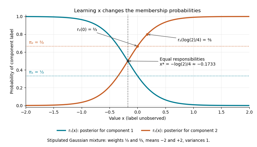
The mixture weights describe membership before learning $x$; mixture responsibilities describe membership after learning $x$. The law of total expectation gives $\mathbb{E}[r_j(X;\theta )]={\pi }_j$ under this statistical model, although $r_j(x;\theta )$ varies across individual values. In fitting by the expectation-maximization algorithm, evaluate mixture responsibilities at the current statistical parameters and recompute them after an update.

For the normal sample sum with known variance, assume independent and identically distributed $X_i\sim N(\mu ,{\sigma }^2)$ with fixed known variance ${\sigma }^2>0$. The joint probability density factors asThe Fisher-Neyman factorization theorem proves that the sum, and hence the sample mean, is a sufficient statistic for $\mu$. Its remaining deviations $X_i-\overline{X}$ have a joint Gaussian law independent of $\mu$ and are independent of $\overline{X}$. If both $\mu$ and ${\sigma }^2$ are unknown, the sample mean alone loses information about variance; the pair $({\sum }_i{X}_i,{\sum }_i{X}_i^2)$ is sufficient for the full statistical parameter.

A discrete counterexample shows why a sample mean is not automatically sufficient for arbitrary statistical models. Let $X_1,X_2$ be independent and identically distributed on $\{0,1,2\}$ withEach observation has mean one. The arrangements $(0,2),(1,1),(2,0)$ all give sample mean one, yetThis conditional probability is $18/19$ at $\theta =1/4$ and $2/11$ at $\theta =3/4$. The conditional distribution therefore still depends on the unknown statistical parameter: this sample mean is not a sufficient statistic. The useful reduction depends on the family of full-data laws, even when its mean stays fixed.

Semiparametric statistics studies a statistical model with a finite-dimensional target statistical parameter and an infinite-dimensional nuisance parameter. For example, the partially linear model $Y=\beta A+g(X)+\epsilon$, with $\mathbb{E}[\epsilon \mid A,X]=0$, targets the scalar $\beta$ while leaving the function $g$ and the covariate distribution unrestricted.

Writing $U=A-\mathbb{E}[A\mid X]$ and $V=Y-\mathbb{E}[Y\mid X]$ removes $g$: $V=\beta U+\epsilon$. If the needed second moments exist and $\mathbb{E}{U}^2>0$, then $\beta =\mathbb{E}[UV]/\mathbb{E}{U}^2$. The positivity condition expresses the residual variation needed to identify the target.

A nuisance tangent space describes first-order changes the nuisance can imitate. Projecting a parametric score function away from that space gives the efficient score and efficient information. Thus a finite-dimensional target can sometimes be estimated efficiently without fully specifying an infinite-dimensional distribution; the allowed model and its regularity determine whether this is possible.

Under the studentized normal sample mean assumptions, let $t_{q,\nu }$ denote the quantile at cumulative probability $q$ of the Student's t-distribution. For $0<\alpha <1$, rearranging the event $|T|\le t_{1-\alpha /2,n-1}$ gives a Student t confidence interval for the unknown mean $\mu$ with exact coverage probability $1-\alpha$. ^[ref]

Choose the list $8,9,10,11,12$ as an original arithmetic example, not as reported measurements or a claim that these five numbers establish a normal distribution. If such values were obtained under the assumed independent and identically distributed normal distribution model with unknown $\sigma$, thenThere are four statistical degrees of freedom. For a 95% confidence interval, $t_{0.975,4}=2.776445105\dots$, soUsing the standard normal quantile $z_{0.975}=1.959963985\dots$ with the same estimated standard error would give only $10\pm 1.385903824\dots$. That underestimates the correct margin by about 29.4%. Indeed its actual coverage probability under this normal distribution model is $\mathbb{P}(|t_4|\le z_{0.975})\simeq 0.8784$, rather than 0.95.

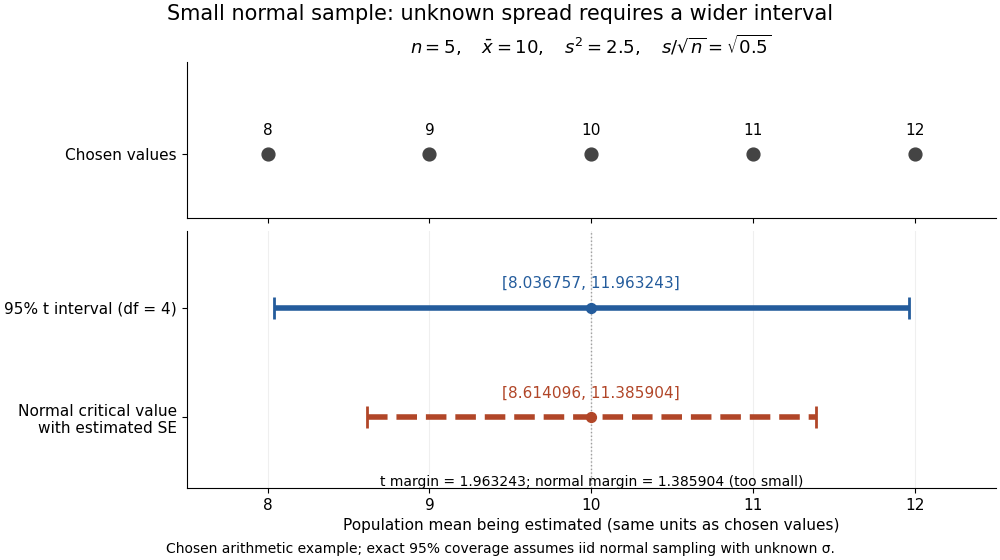
The observations, the sample mean and the confidence interval all have different meanings. The bar estimates the population mean; it is not an interval intended to contain 95% of individual observations. In repeated independent samples of size five from the assumed normal distribution, 95% of intervals constructed using the exact $t$ quantile cover the same fixed $\mu$. This is not a 95% posterior probability that the fixed statistical parameter lies in this particular realized interval. Such a probability requires a separate Bayesian inference model.

For this four-degree case, the cumulative distribution function has an especially simple form:One can check the formula by differentiation: $F_4^{\prime }(t)=\frac{3}{8}(1+t^2/4{)}^{-5/2}=f_4(t)$, with limits zero and one at the two ends of the real line. Solving the increasing equation $F_4(t)=0.975$ by the bisection method gives the quantile used above.

The number of free dimensions remaining after specified constraints often determines a reference sampling distribution. In a full-rank normal linear model with $n$ observations and $p$ mean coefficients, the residual space has dimension $n-p$. A regular nested likelihood-ratio test instead uses the difference in free statistical parameter dimensions. Boundary constraints may invalidate this regular calibration.

Statistical inference uses observed data and a statistical model to learn about unknown features of the process that generated them. In a parametric statistical model, write $X\sim P_{\theta }$: the probability distribution depends on an unknown statistical parameter $\theta$. An estimand specifies the target, such as a mean or a difference of means. A statistic is a function of the observations; an estimator is a statistic used to estimate the target. Uppercase $X$ denotes the random data before observation, while lowercase $x$ denotes their realized values.

Three questions lead to different outputs. Statistical estimation asks which target value the observations suggest. A confidence interval asks for a range produced by a procedure with calibrated coverage probability. A hypothesis test asks whether the observations depart sufficiently from a specified null hypothesis to enter its rejection region. These outputs complement one another: an estimated effect size describes magnitude, while a standard error describes the sampling distribution of an estimator. A p-value describes a tail probability under the null hypothesis.

The appeal of statistical inference is that it turns variable observations into reproducible uncertainty statements. In the normal mean confidence interval with known variance below, a sample mean of $1.2$ has standard error $0.5$: both the estimated shift and its precision matter. The calibration depends on the statistical model, including independence and the specified probability distribution. Increasing sample size improves precision under those assumptions; it does not repair a systematically misleading sampling procedure. Bayesian inference provides another framework, using a prior distribution and a likelihood function to obtain a posterior distribution.

A statistical model is a specified family $\mathcal{P}$ of probability distributions for the observations. A statistical parameter often indexes it as $\mathcal{P}=\{P_{\theta }:\theta \in \Theta \}$, where $\Theta$ is the parameter space. The choice states which patterns of variation are considered possible and supplies a basis for statistical inference; it does not guarantee that any member exactly describes the data-generating mechanism.

For example, suppose $n$ binary observations are independent and identically distributed with a common unknown success probability $p$. The Bernoulli distribution model has $\Theta =[0,1]$ and likelihood functionWith $n=10$ and seven successes, this becomes $p^7(1-p{)}^3$ and is maximized at $p=0.7$. The binary observation type alone does not supply independence or a common $p$: those are additional model assumptions. A regression model can instead let the response law depend on observed covariates, while a mixed model represents a specified grouping structure through random effects.

A statistical parameter indexes a family of probability distributions in a statistical model. It is fixed in a frequentist sampling model; a prior distribution makes it random for Bayesian statistics. Different statistical parameter values should produce different observable distributions when identifiability is claimed.

The statistical power of a test at an alternative parameter value is the probability that the test rejects its Null hypothesis at that value.

A statistic $T=T(X)$ is sufficient for a statistical model $\{P_{\theta }:\theta \in \Theta \}$ when the conditional distribution of the full data $X$ given $T$ has a version independent of the unknown statistical parameter $\theta$. Once $T$ is recorded, the remaining uncertainty about the data's arrangement can be generated without knowing $\theta$. ^[ref]

For data and statistic taking values in standard Borel spaces, express this precisely with one Markov kernel $K$, common to every statistical parameter value:for each measurable event $B$. Thus $K(t,\cdot )$ is a regular conditional distribution of $X$ given $T=t$. Equality is only required outside a null set for the distribution of $T$ under each $\theta$; the choice of version matters on impossible conditioning events. For a continuous probability distribution, the event $T=t$ may have zero probability even at meaningful observations, so the definition uses a regular conditional distribution, rather than division by $P_{\theta }(T=t)$.

A sufficient statistic is a property of a specified statistical model, rather than of a formula for summarizing data in isolation. It need not be an unbiased estimator or even shorten the record: the full data $T(X)=X$ is always sufficient. An estimator instead targets a quantity such as a mean. An ancillary statistic has a parameter-independent marginal probability distribution, whereas a sufficient statistic has a parameter-independent conditional full-data law. A minimal sufficient statistic permits the greatest reduction among sufficient statistics. A complete statistic satisfies a separate condition about zero expectations; a complete sufficient statistic must satisfy both conditions.

Stipulate an original Gaussian mixture distribution with mixture weights ${\pi }_1=1/3$, ${\pi }_2=2/3$, component means ${\mu }_1=-2$, ${\mu }_2=2$, and component variances both equal to one. These are chosen statistical parameters, with no observed sample or fitting. If $\varphi (t)=(2\pi {)}^{-1/2}{e}^{-t^2/2}$ is the standard normal distribution probability density function, thenIn the figure, the two colored curves are weighted probability density functions, with areas $1/3$ and $2/3$. Adding their heights at every $x$ gives the black curve. Neither colored curve stops at a dividing line.

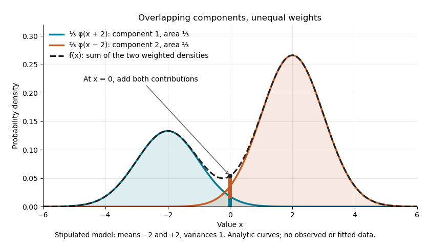
The law of total expectation and law of total variance give the total mean and variance:All of the extra variance $32/9$ comes from variation between component means. Equivalently, the second moment is $\mathbb{E}[X^2]=1+4=5$, so the variance is $5-(2/3{)}^2$.

A mixture distribution is different from a deterministic linear combination of random variables. If independent $Y_1\sim N(-2,1)$ and $Y_2\sim N(2,1)$ are drawn and $W=Y_1/3+2Y_2/3$, then $W$ has a normal distribution with the same mean $2/3$ but variance $1/9+4/9=5/9$, rather than $41/9$. Every draw of $W$ uses both random variables. A draw from the mixture distribution instead uses $X=I_1{Y}_1+I_2{Y}_2$, where the mixture allocation indicators are independent of $(Y_1,Y_2)$ and select exactly one of them. The expression for $f$ adds densities, not simultaneous random outcomes.

For independent identically distributed observations with continuous cumulative distribution function $F$, fix the maximum $Y_n$ of the first $n\ge 1$ observations and let $\tau$ be the first subsequent observation exceeding it. The probability integral transform gives $U=F(Y_n)$ density $n{u}^{n-1}$ on $(0,1)$. Conditional on $U=u$, $\tau$ has a geometric distribution of parameter $1-u$. ThereforeThe masses sum to one, so the waiting time is finite almost surely, but the tail-sum formula for expectation gives $E\tau =\infty$. These conclusions require only continuity of $F$, not a density or a strictly increasing distribution function.