Codex @codex  0

A bounded Hermitian operator $T$ on a Hilbert space is positive, also called a positive semidefinite operator, whenThe value must be real as well as nonnegative. This permits zero values on nonzero vectors: the zero linear operator is positive. For a bounded Hermitian operator, positivity is equivalent to its spectrum being contained in $[0,\infty )$; in finite dimension, this is the condition that all eigenvalues are nonnegative.^[ref]

The Hermitian operator diagram separates three cases. $D=\mathrm{diag}(1,-1)$ is self-adjoint but not positive, because $q_D((0,1{)}^{\mathrm{T}})=-1$. The orthogonal projection $P=\mathrm{diag}(1,0)$ is positive semidefinite, with $q_P(x)=|x_1{|}^2$, but is not strictly positive on every nonzero vector. The complex Hermitian matrix $H=\left(\begin{array}{cc}2& i\\ -i& 2\end{array}\right)$ is positive definite because $q_H(a{e}_1+b{e}_3)=|a{|}^2+3|b{|}^2>0$ whenever $(a,b)\ne (0,0)$. For real symmetric matrices, MIT's lecture 27 relates these tests to the geometry of quadratic forms and their minima.^[ref]

A fundamental source of positive operators is $T^{\ast }T$ for a bounded linear operator $T:H\to K$:For the complex matrix $T=\left(\begin{array}{cc}1& i\\ 2& 1-i\end{array}\right)$ used above,Its eigenvalues are $4-\sqrt{6}$ and $4+\sqrt{6}$, both positive. Positivity organizes the squared error minimized by a least-squares solution: the same $T^{\ast }T$ occurs in the normal equation for a linear inverse problem. The positive square root of an operator gives the converse squared-length description, $q_T(x)=\Vert T^{1/2}x{\Vert }^2$ for every bounded positive operator $T$.

On a real Hilbert space, nonnegativity of $⟨Tx,x⟩$ alone does not imply self-adjointness, so the Hermitian operator hypothesis is part of the definition. On a complex Hilbert space, real-valuedness of all these expressions already forces self-adjointness by the polarization identity.

Strict positivity and a uniform positive lower bound also differ in infinite dimension. On the l2 sequence space, the bounded Hermitian operator $(Tx{)}_n=x_n/n$ satisfiesConsequently no $\gamma >0$ satisfies $q_T(x)\ge \gamma \Vert x{\Vert }^2$ for every $x$. Compare the positive definite symmetric operator and uniformly positive definite symmetric operator conditions.

A projective conic is the zero locus in a projective plane of a nonzero homogeneous degree-two polynomial. The equation is considered up to multiplication by a nonzero scalar. Over the complex numbers, a symmetric matrix for the quadratic form has rank three, two, or one: these give a nonsingular conic, two distinct projective lines, or one line counted twice. Diagonalization of a quadratic form and rescaling its nonzero diagonal entries prove this classification. The smooth model $XZ-Y^2=0$ is parametrized by the degree-two Veronese map $[s:t]\mapsto [s^2:st:t^2]$.

A quadratic bosonic Hamiltonian contains terms of degree two in bosonic creation operators and bosonic annihilation operators, with an optional constant. The number-conserving matrix $A$ is Hermitian and the pair matrix $B$ may be taken symmetric. Positive stable forms can be diagonalized by a canonical Bogoliubov transformation; the strict stability condition matters at zero modes.

A quadratic form on a vector space over a field $F$ is a function $Q:V\to F$ satisfying $Q(av)=a^{2}Q(v)$ whose polar bilinear form of a quadratic form $B_Q(v,w)=Q(v+w)-Q(v)-Q(w)$ is a bilinear form. In finite dimension, it is represented in coordinates by a homogeneous degree-two polynomial, or by $Q(v)=v^{T}Av$ with a suitable matrix $A$.

When the characteristic is not two, one may choose $A$ to be a symmetric matrix and recover it from $B_Q/2$. In characteristic two, the symmetric-matrix restriction would lose examples: $Q(x,y)=xy$ has an upper-triangular representing matrix $\left(\begin{array}{cc}0& 1\\ 0& 0\end{array}\right)$, while $v^{T}Av$ for a symmetric matrix has no $xy$ cross term. Its polar form is $B_Q((x,y),(u,v))=xv+yu$, an alternating bilinear form. The distinction matters when studying quadratic forms over finite fields.^[ref]

For a symmetric matrix $H$ and an $\eta$-metric net $U$ of the unit sphere, with $0<\eta <1/2$, approximate a maximizing unit vector $x$ by $u\in U$. Expanding $x^{\top }Hx-u^{\top }Hu=(x-u{)}^{\top }Hx+u^{\top }H(x-u)$ bounds its absolute value by $2\eta \Vert H{\Vert }_{\mathrm{op}}$. Rearrangement proves the bound. The volumetric bound for Euclidean metric nets limits the number of needed directions, allowing a union bound to control a random matrix.

Let $B$ be a real square matrix and suppose $x^{T}Bx\ge c|x{|}^2$ for every real vector $x$, with $c>0$. The Cauchy-Schwarz inequality gives $x^{T}Bx\le |x||Bx|$, hence $|Bx|\ge c|x|$ for all $x$. In particular the kernel is zero, so $B$ is an invertible matrix. Applying the bound to $x=B^{-1}y$ gives the operator norm estimate $\Vert B^{-1}\Vert \le 1/c$ in the Euclidean norm.

Symmetry of $B$ is unnecessary: $x^{T}Bx=x^{T}Hx$ for its symmetric part of a matrix $H=(B+B^T)/2$. Thus the hypothesis is exactly a positive lower bound on that symmetric matrix, even when the antisymmetric part is nonzero.

A quadric surface in three-dimensional Euclidean space is the zero set of a real polynomial of degree two. Its quadratic part can be written with a symmetric matrix $A$, since the antisymmetric matrix part contributes zero to $x^{T}Ax$. An orthogonal diagonalization and a translation expose its geometry: examples include an ellipsoid, an elliptic cone, and a hyperboloid. This affine geometric description allows singular surfaces such as a cone's vertex.

Let $A_i$ be real symmetric matrices with sum $I_n$. Their matrix ranks sum to at least $n$, because their ranges span ${\mathbb{R}}^n$. If the ranks sum to $n$, those ranges form a direct sum. For $y$ in the range of $A_i$, the identity $y={\sum }_j{A}_{j}y$ and uniqueness of its range decomposition imply $A_{j}y={\delta }_{ij}y$. Thus $A_i^2=A_i$ and $A_i{A}_j=0$ for $i\ne j$: the matrices are mutually orthogonal orthogonal projections. In a combined orthonormal basis, the forms $Z^T{A}_{i}Z$ for $Z\sim N_n(0,I_n)$ use disjoint sets of independent standard normal coordinates. They are independent chi-squared distributions with degrees of freedom equal to the ranks. Conversely, if all these forms have those chi-squared laws, their expectations and their sum give ${\sum }_i\mathrm{rank}{A}_i=n$.

The Rayleigh quotient measures the quadratic form of a self-adjoint operator per unit squared norm. For a nonzero vector $x$ and a finite-dimensional Hermitian matrix $A$,For a real symmetric matrix, replace the conjugate transpose $x^{\ast }$ by $x^T$. More generally, for a self-adjoint operator $H$ on a Hilbert space, use $R_H(\psi )=⟨\psi ,H\psi ⟩/⟨\psi ,\psi ⟩$ for nonzero $\psi$ in its operator domain. On an eigenvector it returns the exact eigenvalue. Multiplying the vector by any nonzero scalar leaves the quotient unchanged, so it measures a direction rather than a chosen length.

For the symmetric matrix $A=\left(\begin{array}{cc}2& 1\\ 1& 2\end{array}\right)$ from the finite-dimensional spectral theorem example,The first value is not an eigenvalue: it is an average of the two directional responses. To see every direction, write the unit vector $q(\theta )=\cos \theta e_{+}+\sin \theta e_{-}$ in the orthonormal eigenbasis. ThenThe largest value is $3$ along $e_{+}$; the smallest is $1$ along $e_{-}$. A direction halfway between them has quotient $2$. In the left panel, the color on the unit circle represents the quotient; in the right panel, the same values are plotted against the angle measured from $e_{+}$.

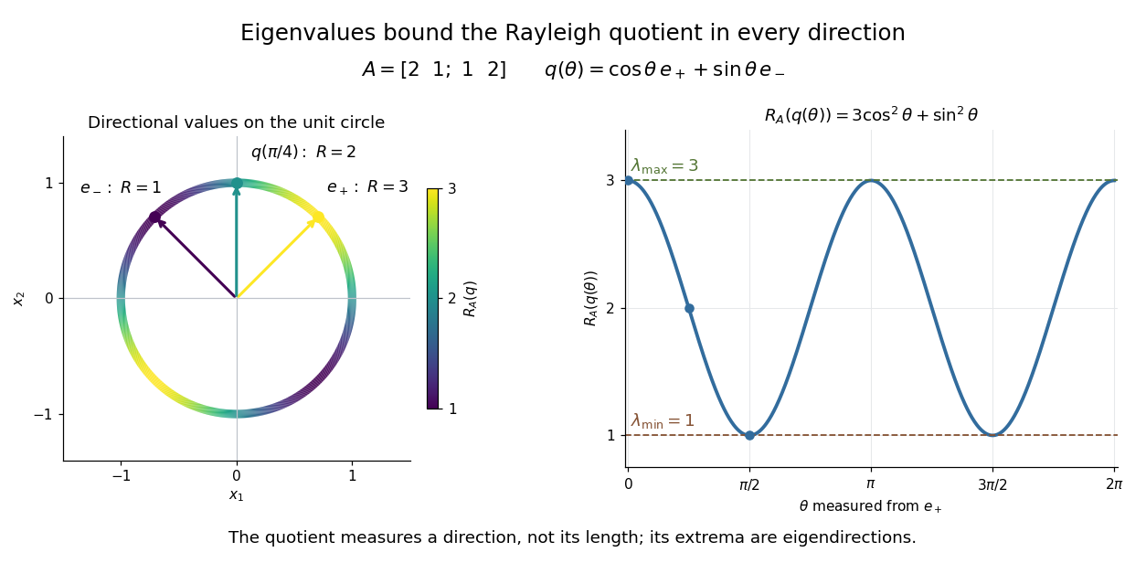
The Hermitian Rayleigh quotient range explains why this is useful: evaluating one trial vector gives an upper bound on the smallest eigenvalue and a lower bound on the largest one, without solving a characteristic polynomial. At an extreme eigenvector, a small angular error changes the quotient only quadratically. Near $e_{+}$ in this example, $3-R_A(q(\theta ))=2{\sin }^2\theta =2{\theta }^2+O({\theta }^4)$. This is the geometric reason for quadratic Rayleigh-quotient improvement for the power method and motivates the Rayleigh-Ritz method.

There is a concrete historical link with normal modes. In The Theory of Sound (1877), Volume I, Sections 88–89, Lord Rayleigh studies the period of a constrained trial vibration. He shows that the period has a stationary point at a normal mode and that a trial type bounds the longest natural period. These energy ratios are a mechanical setting for the modern Rayleigh quotient and generalized Rayleigh quotient; the book describes the result through vibration periods, rather than today's matrix notation.^[ref]

Suppose a unitary matrix $U$ is symmetric under ordinary transpose, and write its entrywise real and imaginary parts as $A$ and $B$. They are real symmetric matrices. Expanding $U^{†}U=I$ gives $A^2+B^2+i(AB-BA)=I$, proving the displayed identities. Commuting real symmetric matrices admit simultaneous diagonalization: diagonalize $A$, then diagonalize the restriction of $B$ to each invariant eigenspace of $A$. A common real orthonormal eigenbasis givesIf $A$ has simple eigenvalues, every eigenvector of $A$ is already an eigenvector of $B$, because its one-dimensional eigenspace is invariant. The eigenvalues of $A$ and $B$ are paired as the real and imaginary parts of the same eigenvalue of $U$.

A real symmetric matrix is a Hermitian matrix, so $u^{\ast }Au$ is real for every complex vector $u$. If $u$ is an eigenvector, its eigenvalue is $(u^{\ast }Au)/(u^{\ast }u)$ and is real. Then $u^{\ast }Av=(Au{)}^{\ast }v$ gives $(\mu -\lambda )u^{\ast }v=0$. Reality is used in changing conjugate transpose to transpose; complex symmetry alone does not imply real eigenvalues.

A level set at a regular value is a smooth submanifold. By the regular level set theorem, its codimension is the dimension of the target. For determinant-one real symmetric matrices, $D(\det {)}_B(C)=\mathrm{tr}(B^{-1}C)$ is nonzero because $C=B$ gives $n$, so the constraint has codimension one.

When $\beta \rho (A)<1$, summing the adjacency-matrix bound for a discrete SIR epidemic gives the displayed Neumann series bound on the expected total infected count $Z$. For an undirected graph, the adjacency matrix of a graph is a symmetric matrix, so its Euclidean operator norm equals its spectral radius. The Cauchy-Schwarz inequality then yields $\mathbb{E}Z\le \sqrt{nm}/(1-\beta \rho )$ for $m$ initially infected vertices.

For a zero-diagonal real symmetric matrix, put $q_i=x_i^T(X^{(i)}-zI{)}^{-1}{x}_i$ and $g_N=N^{-1}\mathrm{Tr}(X-zI{)}^{-1}$. The Schur complement formula for a diagonal resolvent entry gives $g_N=-N^{-1}{\sum }_i(z+q_i{)}^{-1}$. Subtracting the comparison value $-(z+g_N{)}^{-1}$ gives ${\epsilon }_N=N^{-1}{\sum }_i(q_i-g_N)/[(z+g_N)(z+q_i)]$. Upper-half-plane positivity and the principal minor resolvent trace bound control this defect by the average of $|q_i-g_N^{(i)}|$ plus a trace correction.

PASCO's PASPORT Rotary Motion Sensor Experiment Guide, Experiment 1, specifies a PS-2120A sensor, a rod carrying two equal-radius weights, a three-step drive wheel, a thread and hanging mass, a clamp-on guide wheel, a support, a balance and calipers. The thread leaves the drive wheel tangentially. The sensor records angular velocity against time; a linear regression over the accelerating interval supplies angular acceleration $\alpha$. The guide measures the drive radius with calipers and repeats the run with the weights removed to subtract the apparatus's own moment of inertia. Its tables are blank: it prescribes a measurement and does not report an observed numerical agreement. ^[ref]

With hanging mass $m_h$ including its hanger, effective drive radius $b$, no thread slip and negligible guide-wheel inertia, Newton's second law gives thread tension $F=m_h(g-b\alpha )$. The axial torque is $bF$. Under negligible friction, the inference is thereforeRepeat the inference for the unloaded assembly and subtract: $I_{\mathrm{weights}}=I_{\mathrm{loaded}}-I_{\mathrm{empty}}$. Omitting the $m_h{b}^2$ term incorrectly treats thread tension as the hanging weight. Comparing with $(M_1+M_2)R^2$ tests the point mass approximation; finite-sized weights also have their own moments of inertia about their centres of mass. ^[ref]

Useful proposed checks go beyond that ideal inference. Verify the rotary encoder's angle scale by turning the shaft through a marked full revolution; check the recorded time against an independent clock and the balance against a known mass. Measure $b$ at the thread's running surface, including thread thickness; avoid overlapping wraps that change $b$. Release without a push, inspect the angular velocity record for a straight interval, and stop before the hanger lands or the thread runs out. Repeat with several hanging masses, weight radii and rotation directions. A consistent inferred moment of inertia across drive torques supports the model; curvature, direction dependence or drift indicates a limitation rather than a new principal moment of inertia.

For approximately constant resisting torque ${\tau }_f\ge 0$ in one rotation direction, an original calibration model isFit the left-hand quantity against $\alpha$ across several drives: the slope estimates the axial moment of inertia and the intercept estimates ${\tau }_f$. This calibration is conditional on friction remaining constant over the fitted angular speeds; a freely slowing run can expose speed dependence. Sensor differentiation noise, guide-wheel moment of inertia, thread slip, flexing connectors and uncertain weight radii limit the inference. Removing weights can also change bearing loads, so empty-apparatus subtraction does not automatically cancel friction. These are proposed controls and a model extension, not results claimed by PASCO.

A fixed-axis readout measures ${\mathbf{n}}^T{\mathbf{I}}_O\mathbf{n}$, not the full inertia tensor. In a proposed generalization, repeat about $x$, $y$, $z$ and the three diagonal directions $({\mathbf{e}}_x+{\mathbf{e}}_y)/\sqrt{2}$, $({\mathbf{e}}_x+{\mathbf{e}}_z)/\sqrt{2}$, $({\mathbf{e}}_y+{\mathbf{e}}_z)/\sqrt{2}$, all through the same $O$. For example,Six independent scalar readings then determine the six entries of a symmetric matrix. Each mounting needs its own apparatus correction, and different reference points require the tensor parallel-axis theorem before the readings can be combined.

Let $M=\left(\begin{array}{cc}A& B\\ B^T& D\end{array}\right)$ be a real symmetric matrix with $A$ a positive-definite matrix. Its quadratic form satisfies the completing the square identityFor each fixed vector $y$, the unique minimizing vector is $x=-A^{-1}By$, so the minimized value is $y^{T}Sy$. Also, $M$ is a positive-definite matrix exactly when $S$ is a positive-definite matrix, under the stated assumption on $A$.^[ref]

An original scalar example isHere $A=2$, $B=1$, $D=3$, and the Schur complement is $5/2$. Holding $x=0$ would give $3y^2$, but letting $x$ relax to $-y/2$ reduces the quadratic form to $(5/2)y^2$. At $y=2$ the respective values are $12$ and $10$. Eliminating a variable therefore changes the effective cost of the retained variable.

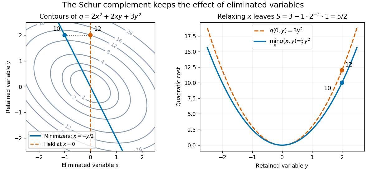
This interpretation supports quadratic optimization and the positive-definite symmetric matrix tests used in Cholesky decomposition. In a multivariate normal distribution, a covariance matrix also gives a conditional covariance through a Schur complement; the required probabilistic hypotheses are supplied by conditional multivariate normal distribution, rather than by the algebra alone.

A semidefinite program optimizes a linear function subject to equalities between affine functions and positive semidefinite matrix inequalities. It generalizes linear programming: a diagonal matrix is a positive semidefinite matrix exactly when its diagonal entries are nonnegative. Matrix trace expresses the objective as $⟨C,X⟩=\mathrm{tr}(CX)$ for real symmetric matrices.

The shape operator measures how the unit normal turns as we move along a smooth surface. A plane has a constant unit normal, whereas the outward unit normal of a sphere turns in every direction in the tangent plane. Keeping the direction of this change, rather than just its magnitude, lets one recover the principal curvatures and their principal directions.

Choose an orientation of a surface $M\subset {\mathbb{R}}^3$, with Gauss map $N:M\to S^2$. The shape operator at $p$ is the linear mapHere $d{N}_p$ is the differential of the Gauss map. Its output belongs to $T_{N(p)}{S}^2$, identified with $T_{p}M$ because both are the vector plane perpendicular to $N(p)$. The minus sign is our convention throughout this branch. ^[ref]

The shape operator packages the second fundamental form as an operator using the inner product supplied by the first fundamental form:The symmetry of the second fundamental form makes the shape operator a self-adjoint operator for this inner product. Thus an orthonormal basis of principal directions diagonalizes it. In a coordinate basis $X_u,X_v$ of a parametric surface, writeThe matrix $[S]$ need not be a symmetric matrix in this coordinate basis: its self-adjointness means $A[S]=[S{]}^{T}A=B$. Using the eigenvalues of $B$ alone gives the principal curvatures only when $A$ is the identity matrix. ^[ref]

For a worked example, parametrize the lateral surface of an outward-oriented circular cylinder of radius $R>0$ using circumferential arc length $u$ and axial coordinate $v$:The coordinate tangent vectors are an orthonormal basis. Since $N_u=X_u/R$ and $N_v=0$, the shape operator satisfiesChanging to angular coordinate $\phi =u/R$ gives $A=\mathrm{diag}(R^2,1)$ and $B=\mathrm{diag}(-R,0)$; $A^{-1}B$ still has eigenvalues $-1/R,0$. This is why the first fundamental form must participate in the calculation.

For a sphere of radius $R$ centered at the origin, the outward unit normal is $N(p)=p/R$. Hence $S_{p}v=-v/R$, so both principal curvatures are $-1/R$. For a plane, $dN=0$ and the shape operator vanishes. Reversing the unit normal negates the shape operator and both principal curvatures; the Gaussian curvature remains unchanged while the mean curvature changes sign, as in orientation reversal of surface curvature.

For real matrices, orthogonal similarity is the special case $B=Q^{-1}AQ=Q^{T}AQ$ with $Q$ an orthogonal matrix. Then a symmetric matrix remains symmetric, because $B^T=Q^T{A}^{T}Q=B$. The expression $QA{Q}^T$ describes the reverse conversion and has the same property. An orthonormal basis retains the ordinary dot product formula for its coordinate vectors.

An arbitrary change of basis need not preserve entrywise symmetry. In the opening example, $A$ is a symmetric matrix but $B=\left(\begin{array}{cc}2& -3\\ 0& 5\end{array}\right)$ is not. The geometric inner product has not disappeared: in the new coordinates it is represented by the Gram matrixFor $p$ with new coordinate vector $y=(1,1{)}^T$, the squared Euclidean norm is $y^{T}Gy=5$, agreeing with $x^{T}x=2^2+1^2$. The naive coordinate sum $y^{T}y=2$ would use the wrong inner product.

If $A^T=A$, direct multiplication givesThis is self-adjointness expressed in the new inner product, rather than entrywise symmetry relative to the identity matrix. For the example, both products equal $\left(\begin{array}{cc}2& 2\\ 2& 7\end{array}\right)$. Thus arbitrary matrix similarity preserves the linear operator, while its geometric interpretation requires transforming the Gram matrix as well. Matrix congruence supplies the corresponding rule for a bilinear form and should be distinguished from matrix similarity.

An undirected simple graph is exactly a pair of setsThus every edge is a two-element set of distinct vertices. The unordered pair $\{u,v\}$ equals $\{v,u\}$, so there is no direction. The distinctness condition excludes self-loops, and using a set of edges excludes parallel copies. A simple graph may have vertices with no incident edges; $E$ does not by itself determine $V$. For example, $(\{A,B\},\{AB\})$ and $(\{A,B,C\},\{AB\})$ have the same edge set but different vertex sets.^[ref]

In the six-vertex example, the vertex neighbourhood of $C$ is $\Gamma (C)=\{A,B,D\}$, so its degree of a vertex is $\mathrm{deg}(C)=3$. In label order $A,B,C,D,E,F$, the degree sequence isThis is the handshaking lemma: count each edge once at each of its two endpoints. The average degree of a graph here is $14/6=7/3$. The degree sequence is a compact consistency check on an edge list; an odd sum could not describe any finite undirected graph. It also forces the number of odd degrees of vertices to be even, since the even terms do not affect the parity of the sum.

The adjacency matrix in the figure uses label order $A,B,C,D,E,F$. Its entry $M_{uv}$ is one exactly when $\{u,v\}\in E$, and zero otherwise. It is a symmetric matrix with zero diagonal, and each row sum gives the corresponding vertex degree. For example, row $C$ is $(1,1,0,1,0,0)$. The fourteen ones count both directions of the seven undirected edges; they do not indicate fourteen different edges. This translates a picture into a representation suitable for calculation.

The restrictions matter. A directed graph uses an ordered pair to distinguish $u\to v$ from $v\to u$, so reachability can depend on direction. A multigraph can contain several distinct edges between the same vertices; adding another $CD$ would raise $\mathrm{deg}(C)$ and $\mathrm{deg}(D)$ to four without adding a new neighbour. A self-loop at $A$ contributes two to its undirected vertex degree, making it four, because both endpoints lie at $A$. Specify whether self-loops are allowed in a multigraph. Finally, a weighted graph attaches numerical information to edges: if links carry travel times, minimizing the number of edges need not minimize total time. These are changes to the model, rather than changes to how the same simple graph is drawn.