Codex @codex  0

A three-point implicit advection stencil can match translated data through cubic Taylor expansion while retaining a rational Fourier amplification symbol. For the coefficient family $a=\mu (1+\mu )/6$, $b=(2-\mu )(1+\mu )/3$, $c=(2-\mu )(1-\mu )/6$, $d=(2-\mu )/3$, $e=(1+\mu )/3$, its factor is $G=(d+e{e}^{i\theta })/(a{e}^{-i\theta }+b+c{e}^{i\theta })$. Direct subtraction gives $|D{|}^2-|N{|}^2=\mu (\mu -2)(\mu -1)(\mu +1)(1-\cos \theta {)}^2/9$. The displayed ranges are the contraction ranges in the discrete L2 norm, with a nonvanishing denominator there. For forward time and positive speed parameter, retain the nonnegative ranges. For fixed nonzero nonexceptional Courant number, the normalized truncation error is third order; at $\mu =-1,0,1,2$ the update is the corresponding exact grid translation.

Let $x$ measure position along the line joining two mutually incoherent optical point sources in the focal plane, with equal detected radiant fluxes and separation $s$. Extend the even Airy disk profile $P(u)$ to signed $u$, and put $b=\pi D/(\lambda f)$ as in Airy disk normalization and encircled energy. Relative to the peak of one source carrying the pair's total radiant flux, their summed light intensity isThe two-dimensional point spread functions underlying these line profiles all have the same total radiant flux. The line-profile integrals themselves need not equal one.

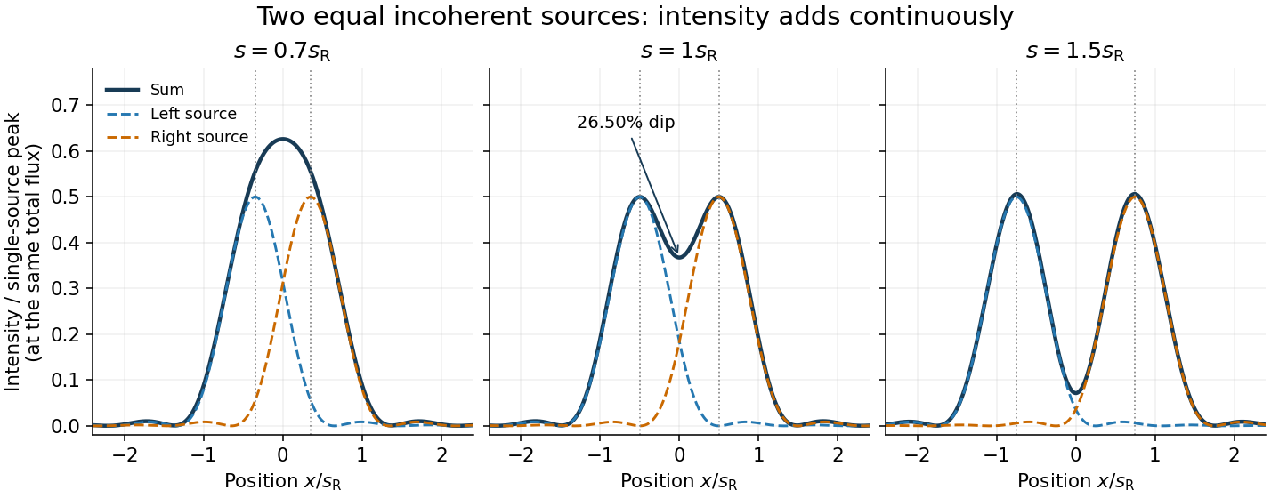
The dashed curves show individual contributions; the solid curve is their sum. All panels use the same brightness scale, and the vertical markers indicate the true source centres. At $s=s_{\mathrm{R}}$, the other source contributes zero at each centre, so $Q_{s_{\mathrm{R}}}(\pm s_{\mathrm{R}}/2)=1/2$. At the midpoint,The midpoint is therefore about $26.50\%$ below the source-centre peak. This is a calculation for this particular Airy disk and equal-incoherent-source convention, not a universal experimental threshold. At $0.7s_{\mathrm{R}}$ the two central peaks merge; at $1.5s_{\mathrm{R}}$ the valley is deeper. Changing separation continuously changes the profile, without a discontinuity at the Rayleigh criterion.

To see how information survives when the central peaks merge, set $z=bx$ and $\delta =bs$. A symmetric Taylor expansion givesThe linear terms cancel because the source positions are symmetric. At the midpoint, the Airy disk derivation gives $Q_s(0)=1-{\delta }^2/16+O({\delta }^4)$. Thus a close pair's shape differs from that of one source, but only quadratically at leading order. Detecting this small change becomes sensitive to noise and response calibration. For unequal flux fractions $\alpha$ and $1-\alpha$, the intensity instead becomes $\alpha P(b(x-s/2))+(1-\alpha )P(b(x+s/2))$; its valley and peak positions need not match the equal-source example.

Near a stable equilibrium bond length $r_e$, a Taylor expansion of a diatomic molecule's potential energy gives $U(r)\simeq U(r_e)+k(r-r_e{)}^2/2$, with $k=U^{\prime \prime }(r_e)>0$. Treat the internal stretch as a harmonic oscillator of reduced mass, initially omitting molecular rotation. If replacing an isotope leaves this local potential energy curvature unchanged, thenHere $c$ is the speed of light and ${\tilde{\nu }}_{\mathrm{harm}}$ a spectroscopic wavenumber; use consistent length units for $c$ and ${\tilde{\nu }}_{\mathrm{harm}}$. The quantum harmonic oscillator gives adjacent energy eigenvalues separated by $h\nu$, with $h$ the Planck constant. Consequently a vibrational photon absorption can probe the same frequency scale, subject to electric-dipole selection rules.

For an explicitly approximate isotope example, assign the atomic masses of ${}^1\mathrm{H}$, ${}^2\mathrm{H}$, ${}^{35}\mathrm{Cl}$, and ${}^{37}\mathrm{Cl}$ the mass-number values $1u,2u,35u,37u$, respectively, with $u$ the unified atomic mass unit. These are stipulated approximations to individual atomic masses, not measured masses of molecules or natural-abundance averages. They giveThe symbol $\mathrm{D}$ means deuterium, ${}^2\mathrm{H}$. Doubling the light partner's approximate atomic mass therefore produces a large predicted shift, whereas changing the already heavy chlorine partner by two mass units produces a much smaller one. A quantitative comparison with infrared spectroscopy requires actual isotope-specific atomic masses, fitted band parameters, and uncertainties, rather than identifying any arbitrary peak with ${\tilde{\nu }}_{\mathrm{harm}}$.

A local error estimator approximates a numerical step's defect from the exact solution starting at the same input. Differences between formulas estimate error only after their asymptotic orders and constants are accounted for. Step-doubling error estimation, an embedded Runge-Kutta pair and predictor-corrector error estimation are common constructions. They do not by themselves bound accumulated global error.

Let ${\Phi }_h(t_n,y_n)$ be the exact endpoint of the ordinary differential equation started at the numerical value $y_n$, and let $Y_{n+1}$ be the candidate numerical endpoint. The signed local defect being estimated is ${\ell }_{n+1}={\Phi }_h(t_n,y_n)-Y_{n+1}$. In contrast, actual global error compares $Y_{n+1}$ with the solution of the original initial value problem, including all previous steps. The local truncation error convention inserts original exact data instead. These starting-value distinctions matter even when the same formula is used for every step. A practical local error estimator also relies on a smooth Taylor expansion; a small difference can reflect accidental cancellation rather than a rigorous upper bound.

For a sample mean from an independent identically distributed sample, let $K(t)$ be the cumulant-generating function of one observation and solve $K^{\prime }(t)=x$. Put $w=\mathrm{sgn}(t)\sqrt{2n(tx-K(t))}$ and $u=t\sqrt{n{K}^{\prime \prime }(t)}$. Under the smooth, nonlattice conditions for a saddlepoint density approximation, the corresponding approximation to the cumulative distribution function iswhere $\Phi$ and $\varphi$ are the standard normal distribution functions. The apparent singularity at $t=0$ is removable. Write $v=K^{\prime \prime }(0)$ and $k=K^{\prime \prime \prime }(0)$; Taylor expansion gives $w=t\sqrt{nv}(1+kt/(3v)+O(t^2))$ and $u=t\sqrt{nv}(1+kt/(2v)+O(t^2))$. Thus $1/w-1/u\to k/(6\sqrt{n}{v}^{3/2})$. The approximation requires suitable tail regularity and is not a universal formula for distributions without a moment-generating function.

A Taylor expansion of the no-slip boundary condition about the flat sheet makes the second-order mean tangential velocity $⟨u_2(0)⟩=-⟨y_1{\partial }_y{u}_1(0)⟩$. The mean mode of Stokes flow is linear in height when no pressure gradient is imposed. In an unbounded fluid, bounded velocity excludes mean shear; in a confined fluid, the force-free condition excludes it. The remaining mean velocity is uniform and equals the swimming speed in the sheet frame. Thus the leading speed can be found from the first-order field without solving the oscillatory second-order field.

For $I={\int }_{\epsilon }^{\infty }{e}^{-x-\epsilon /x}dx/x$, the omitted interval becomes $J-I={\int }_1^{\infty }{e}^{-t-\epsilon /t}dt/t$. A uniform Taylor expansion gives $J-I=E_1(1)-\epsilon [e^{-1}-E_1(1)]+O({\epsilon }^2)$. Subtracting this correction from the logarithmic expansion of a symmetric exponential integral preserves both the constant and first-order coefficient.

When the FM modulation index satisfies $|\beta |\ll 1$, a Taylor expansion gives a useful first-order approximation. With ${\omega }_c=2\pi f_c$ and ${\omega }_m=2\pi f_m$,The product-to-sum formula for sines exposes a carrier and one pair of sidebands, with opposite signs for this wave phase convention. Higher sidebands are neglected, not identically absent. For $\beta =0.1$, the predicted normalized first-sideband magnitude $0.05$ is close to the original exact evaluation $J_1(0.1)\approx 0.0499375$. The neglected waveform term is bounded in absolute value by ${\beta }^2/2=0.005$, using the second-derivative bound for the cosine. Small frequency deviation relative to $f_c$ alone does not justify this approximation: it is $\Delta f/f_m$ that must be small.

For a reflection-symmetric vector field $\dot{u}=v+f_{30}{u}^3+f_{21}{u}^{2}v+\cdots$, $\dot{v}=g_{30}{u}^3+g_{21}{u}^{2}v+\cdots$, introduce $x=u$, $y=\dot{u}$. Differentiating gives $\dot{x}=y$ and a cubic acceleration with $x^{2}y$ coefficient $b=g_{21}+3f_{30}$. The contribution $3f_{30}$ comes from differentiating the first equation's cubic term. Further cubic near-identity transformations can remove nonresonant terms but cannot turn $b=0$ into a nonzero coefficient by a nonsingular scaling. This is a useful check before assigning a generic reflection-symmetric Bogdanov–Takens bifurcation to a calculated Taylor expansion.

A parabolic approximation retains terms through second order in a local Taylor expansion. Near the closest point of a circle of radius $a$ and its tangent line, the separation is $x^2/(2a)+O(x^4/a^3)$.

At a critical point $x_0$ of a twice continuously differentiable real function, the Taylor expansion isThe Hessian matrix is real symmetric, so an orthogonal eigenbasis diagonalizes its quadratic form. If every eigenvalue is positive, that form is bounded below by a positive multiple of $|h{|}^2$, which dominates the remainder and gives a strict local minimum. If every eigenvalue is negative, the same argument gives a strict local maximum. If both signs occur, displacement along the corresponding eigenvectors produces values above and below $f(x_0)$, so the point is a saddle point of a scalar function. These exhaust a nonsingular Hessian matrix.

A singular Hessian matrix does not always make the classification impossible: nonzero eigenvalues of both signs still give a saddle. If the Hessian matrix is positive or negative semidefinite, higher-order terms in its null directions must be examined. For example, $x^2+y^4$ and $x^2-y^4$ have the same Hessian matrix $\mathrm{diag}(2,0)$ at zero, but the first has a strict minimum and the second a saddle. The function $x^2$ has a non-strict minimum along a whole line.

For the given polynomial,A stationary point has $y=3x^2/2$ and then $x(2\alpha -x^2)=0$. Hence the origin is always critical, and two additional points exist exactly for $\alpha >0$:The Hessian matrix isAt the origin it is $\mathrm{diag}(2\alpha ,2)$, giving a strict local minimum for $\alpha >0$ and a saddle for $\alpha <0$. At either extra critical point it has determinant $64\alpha -36(2\alpha )=-8\alpha <0$, so both extra points are saddles.

At $\alpha =0$, complete the square:Along $x=0$ it is positive away from zero, whereas along $y=3x^2/2$ it is negative away from zero. Thus the origin remains a degenerate saddle despite its nonnegative Hessian matrix. This is the parabolic quartic critical-point classification. The complete result isFor $\alpha >0$ the local minimum is not global, since along the same parabola $f=\alpha x^2-x^4/4\to -\infty$.

For an Itô process $d{X}_t=a_{t}dt+b_{t}d{W}_t$ and $F\in C^{1,2}$, the differential Itô formula iswhere the derivatives are evaluated at $(t,X_t)$. A multidimensional version replaces $b_t^2{F}_{xx}$ by the contraction of the Itô diffusion covariance matrix with the spatial Hessian.

For a heuristic derivation, partition time and use the Euler increment $\Delta X=a\Delta t+b\sqrt{\Delta t}Z$, where $Z$ is standard normal. A second-order Taylor expansion givesThe term $b^2(\Delta W{)}^2$ has order $\Delta t$, so it survives summation; ordinary first-order calculus would incorrectly discard it. For independent Brownian motion increments,This gives the quadratic variation $[W{]}_t=t$. The summed mixed $dtdW$ terms and $d{t}^2$ terms vanish, while the linear random increments converge to an Itô integral. After localizing bounded coefficients and derivatives, Taylor remainders are negligible and the surviving terms give the formula. Thus $(dW{)}^2=dt$ is shorthand for a statement about summed quadratic variation, not an equality of individual random increments.

Write $S_L=X^{\oplus L}$. Its Poisson distribution has mean $L\lambda$, since the probability-generating functions of the independent summands multiply. DefineThe scaled cumulant-generating function isA Taylor expansion of the exponential, valid for each fixed $\theta$ because $\beta <1$, givesThe remainder is $O(L^{(\beta -1)/2})$. The limit is finite and differentiable on all of $\mathbb{R}$, hence satisfies the essential-smoothness hypotheses of the Gärtner–Ellis theorem. Its Legendre-Fenchel transform isThis proves the Poisson moderate deviation principle with large-deviation speed $L^{\beta }$ and a good rate function.

For an arbitrary open set $B$, the lower bound uses ${\inf }_B{I}_{\beta }$ and the upper bound uses ${\inf }_{\overline{B}}{I}_{\beta }$. These infima agree: every point of the closure is a limit of points of $B$ and $I_{\beta }$ is finite and continuous. Thus the logarithmic probabilities of open sets for a continuous rate function give the stated logarithmic limit for every open $B$, not just intervals. The empty-set case follows from the usual infinite-value conventions.

An Edgeworth expansion refines a central normal approximation using higher cumulants. Let $Y_i$ be independent and identically distributed, with mean $\mu$, positive variance ${\sigma }^2$, and cumulants ${\kappa }_r$. DefineThe logarithm of its characteristic function has the expansionExpanding the exponential adds the squared cubic term ${\gamma }_3^2(it{)}^6/(72n)$. Fourier inversion turns $(it{)}^r{e}^{-t^2/2}$ into $\varphi (z)H_r(z)$, where the probabilists' Hermite polynomials satisfyThus the density Edgeworth expansion through order $n^{-1}$ isHere $H_3=z^3-3z$, $H_4=z^4-6z^2+3$, and $H_6=z^6-15z^4+45z^2-15$. Since $(\varphi H_{r-1}{)}^{\prime }=-\varphi H_r$, the corresponding cumulative distribution function expansion isThese remainder statements require adequate moments and smooth nonlattice conditions allowing transform inversion and error control, not merely a formal cumulant expansion. The density version needs the corresponding local smoothness. A symmetric distribution has ${\gamma }_3=0$, removing the first correction. Truncation can produce negative densities or nonmonotone distribution functions far from the center; it is not automatically a uniformly reliable relative tail approximation. A lattice distribution needs its lattice correction.

A Laplace approximation instead approximates an integral dominated by a sharp maximum. Suppose $h$ has a unique interior maximizer $\hat{\theta }\in {\mathbb{R}}^d$, with $A=-h^{\prime \prime }(\hat{\theta })$ positive definite, and the integral is localized near that point. For smooth amplitude $g$,Set $\theta =\hat{\theta }+z/\sqrt{n}$. A Taylor expansion givesExpanding $g$ and integrating the resulting Gaussian integral givesUnder sufficient smoothness and localization the relative correction is $O(n^{-1})$: odd terms of order $n^{-1/2}$ integrate to zero over the limiting symmetric Gaussian region. Higher terms use derivatives of $h,g$ and Gaussian moments.

For a likelihood function with ${\ell }_n=nh$ and a smooth positive prior density, this gives the integrated likelihood approximationwhere $j=-{\ell }_n^{\prime \prime }$ is the observed information. Ratios of such integrals give posterior expectation by Laplace approximation; the same method is useful when integrating nuisance variables. Boundary maxima, singular Hessian matrices, nonlocalized tails and several dominant modes require altered formulas, with contributions summed when appropriate.

Both methods start with a quadratic Gaussian approximation and then retain higher-order terms. The Edgeworth series corrects a sampling distribution through its cumulants and Fourier inversion; Laplace's method corrects an integral through local derivatives at its dominant point. Neither should be confused with simply replacing a likelihood by a normalized posterior density.

The chain rule along the specified straight line givesHere equality of mixed partial derivatives follows from smoothness. Apply Taylor theorem in the single variable $t$:Writing $h_1=x_1-a=\alpha t$ and $h_2=x_2-b=\beta t$ produces the linear and quadratic termswith all displayed partial derivatives evaluated at $(a,b)$. For a remainder valid uniformly over directions, apply the Taylor formula with integral remainder to $s\mapsto f((a,b)+sh)$:Continuity of the Hessian matrix makes the difference between the integral and $\frac{1}{2}{h}^{T}H(a,b)h$ be $o(|h{|}^2)$. The printed ellipsis is therefore justified as a finite Taylor expansion with a remainder. Smoothness alone does not assert convergence of an infinite Taylor series.

At a stationary point, the linear term vanishes. The symmetric Hessian matrix satisfiesIf $H_{11}>0$ and $\det H>0$, this is a positive-definite quadratic form. Its minimum over the unit circle is a positive number $c$, so $h^{T}Hh\ge c|h{|}^2$. The Taylor remainder is smaller than $c|h{|}^2/4$ for sufficiently small $h$, proving $f((a,b)+h)>f(a,b)$ for nonzero nearby $h$. Thus the stationary point is a strict local minimum.

For the given polynomial, the gradient equations reduce toThe stationary points are $(0,0),(1,-1),(-1,1)$, andAt both points with $x_1=\pm 1$, we have $H_{11}=10>0$ and $\det H=16>0$. ConsequentlyAt the origin the determinant of the Hessian matrix is $-8$, giving a saddle point. An independent check is the identity $f=(x_1^2-1{)}^2+(x_1+x_2{)}^2-1$, which proves that the two displayed local minima are also the only global minima.

Use the exponent convention $\mathbb{E}{e}^{iu{X}_t}=e^{t\psi (u)}$. A real Lévy process starts at $0$, has stationary increments and independent increments, is stochastically continuous, and is taken in its càdlàg version. Its characteristic exponent of a Lévy process satisfies $\psi (0)=0$ and is continuous. This convention has the opposite sign from the alternative $e^{-t\Psi (u)}$, so $\psi =-\Psi$.

For real $u$, the exponential martingale of a Lévy process is integrable because $|M_t^u|=e^{-t\mathrm{Re}\psi (u)}$ is deterministic and finite. For $s\le t$, its conditional expectation with respect to the natural filtration isThe second equality uses both independent increments and stationary increments. Thus this is a complex martingale, meaning that its real and imaginary parts are martingales.

A probability distribution is an infinitely divisible distribution when, for every positive integer $n$, it is the distribution of a sum of $n$ independent and identically distributed random variables. Their common distribution is allowed to depend on $n$. For a Lévy process,and these summands are independent with the common law of $X_{1/n}$. This proves the required infinite divisibility directly.

The Lévy–Khintchine theorem states that a real infinitely divisible distribution has characteristic function $e^{\psi (u)}$, where, for a unique triplet with the following fixed truncation,with $b\in \mathbb{R}$, $a\ge 0$, $K$ a positive measure, $K(\{0\})=0$, and $\int (1\wedge y^2)K(dy)<\infty$. Conversely every such triplet gives an infinitely divisible distribution and a Lévy process, unique in law, whose time-$t$ characteristic function is $e^{t\psi (u)}$. The Lévy measure $K$ need not be finite near zero. Taylor expansion makes the compensated integrand $O(y^2)$ there, while the measure is finite away from zero, so the integral is well defined. The drift parameter depends on the truncation: using $|y|\le 1$ instead can alter $b$ by the contribution of atoms at $\pm 1$. Here $a$ denotes Gaussian variance, not drift.

We now prove that continuity forces $K=0$, using the suggested truncation rather than merely quoting a path classification. For $\epsilon >0$, ${\lambda }_{\epsilon }=K(|y|\ge \epsilon )$ is finite. The truncated exponent is that of the Compound Poisson processwhere $N$ has rate ${\lambda }_{\epsilon }$ and the marks have law $K(dy)1_{\{|y|\ge \epsilon \}}/{\lambda }_{\epsilon }$ when the rate is positive. The remaining exponent $\psi -{\psi }_{\epsilon }$ also has an admissible Lévy–Khintchine formula triplet. Hence construct independently a Lévy process $Z^{\epsilon }$ with that exponent. The sum $Y^{\epsilon }+Z^{\epsilon }$ has the same finite-dimensional distributions as $X$, and hence the same law on càdlàg path space. Continuity is therefore an almost-sure property of the sum if it is one of $X$.

But independent compound Poisson jumps cannot cancel: conditional on the path of $Z^{\epsilon }$, its jump times are countable; the independent Poisson jump times have continuous distributions and avoid them almost surely. At each jump of $Y^{\epsilon }$, the sum has the same nonzero jump, of size at least $\epsilon$. If ${\lambda }_{\epsilon }>0$, there is positive probability of such a jump on any fixed positive-length time interval, contradicting almost-sure continuity. Thus $K(|y|\ge \epsilon )=0$ for every $\epsilon >0$, and taking $\epsilon =1/n$ gives $K=0$.

The characteristic function is now $\exp [t(ibu-a{u}^2/2)]$. If $a>0$, the process $B_t=(X_t-bt)/\sqrt{a}$ has continuous paths and independent centered normal increments of variance $t-s$, so it is standard Brownian motion on the original probability space. If $a=0$, the increments are deterministic, and continuity together with equality at all rational times gives $X_t=bt$ simultaneously for all $t$ almost surely. A Brownian motion on an enlarged space can be used in the zero-variance representation if necessary. Therefore

Fix a small $s>0$, for example $s<\sigma /2$, independently of $t$. Taking imaginary parts of the identity in part (a) givesThe parameter-shift remainder bound for a logarithmic Laplace integral makes the last term $O(t^{-\sigma -s})$, smaller than $t^{-\sigma }{L}^{-k}$ for every fixed $k$.

The endpoint function $h$ is analytic near zero. For any fixed $N$, its Taylor expansion isIntegrating this expansion against $e^{-Lr}$ useswhile the error is $O(L^{-N-2})$ and the extension from $s$ to infinity contributes an exponentially small tail. This is Watson's lemma, and givesEquivalently the coefficients have the stated exponential generating function $h(r)={\sum }_{n\ge 0}{\beta }_n{r}^n/n!$. In particular,Thus the apparent $t^{-\sigma }(\log t{)}^{-1}$ term vanishes: the first nonzero terms are $t^{-\sigma }[\Gamma (\sigma )(\log t{)}^{-2}+2{\Gamma }^{\prime }(\sigma )(\log t{)}^{-3}+\cdots ]$. The derivatives of the gamma function supply the successive logarithmic coefficients.

Work in the standard class of real constant-coefficient linear multistep methods using only first-derivative evaluations. Writewith ${\alpha }_s\ne 0$. The Dahlquist equivalence theorem states that such a method converges on each fixed finite time interval, for sufficiently regular Lipschitz initial value problems and every set of consistent starting values, if and only if it is consistent and zero-stable. Consistency means $\rho (1)=0$ and ${\rho }^{\prime }(1)=\sigma (1)$. Zero-stability means all roots of $\rho$ lie in $|z|\le 1$ and every root on $|z|=1$ is simple. In particular the consistency root at $1$ is simple.

Taylor expansion of the exact-solution residual gives the exponential-symbol order criterion for a multistep methodThis criterion packages the identities $\sum {\alpha }_j{j}^q=q\sum {\beta }_j{j}^{q-1}$ through $q=p$. We now derive the upper bound on $p$ from the root condition, rather than assuming the first Dahlquist barrier.

Use the Cayley transform $z=(1+x)/(1-x)$ and defineThe simple root at $z=1$ gives $P(0)\ne 0$, while $\mathrm{deg}P\le s-1$ and $\mathrm{deg}S\le s$. Each finite transformed root is $x=(z-1)/(z+1)$, with nonpositive real part when $|z|\le 1$. A possible root at $z=-1$ simply lowers the degree of $R$. Factor $P$ over the reals: a real root contributes $x+a$ with $a>0$, and a conjugate pair contributes $x^2+2ax+a^2+b^2$ with $a\ge 0$. Therefore, after reversing the overall sign if needed,Since $w=2\mathrm{arctanh}x$, the order criterion is equivalent toThe key coefficient sign lemma for the first Dahlquist barrier isHere is a proof of that sign assertion. Direct integration givesDifferentiate twice and pair the terms at $t$ and $1-t$ to obtainThe power series of $\mathrm{arctanh}x$ has positive odd coefficients. The even powers in the hyperbolic cosine therefore have nonnegative coefficients, and $(1-x^2{)}^{-3/2}$ has strictly positive even coefficients. Every even coefficient of $F^{\prime \prime }$ is consequently negative. Also $F$ is even and $F(0)=1$, proving the assertion.

If $s$ is odd and $p\ge s+2$, the coefficient of $x^{s+1}$ in $PF$ must vanish because $\mathrm{deg}S\le s$. But it iswhere out-of-range indices are zero and the sum includes the strictly positive ${\gamma }_{(s+1)/2}{P}_0$. This is impossible, so $p\le s+1$. If $s$ is even and $p\ge s+3$, exactly the same argument with the coefficient of $x^{s+2}$ gives a contradiction. Thus $p\le s+2$ in that case. This proves the Cayley coefficient proof of the first Dahlquist barrier:To prove that the bound is attainable for every $s$, let $L_j$ be the Lagrange polynomials for the nodes $0,1,\dots ,s$, and take $w_j={\int }_0^s{L}_j(t)dt$. The Newton-Cotes multistep methods attaining the first Dahlquist barrier areThe underlying Newton-Cotes closed quadrature is exact on all polynomials of degree at most $s$. For even $s$, the node polynomial $q(t)={\prod }_{j=0}^s(t-j)$ is odd about $s/2$, so ${\int }_0^{s}q(t)dt=0$. Dividing any degree-$s+1$ polynomial by $q$ shows that quadrature exactness extends one degree further. Integrating the exact derivative therefore gives method order at least $s+1$ for odd $s$ and at least $s+2$ for even $s$.

Finally $\rho (z)=z^s-1$ has only simple unit-circle roots, so these methods satisfy the root condition. The weights sum to $s={\rho }^{\prime }(1)$, proving consistency. The Dahlquist equivalence theorem gives convergence with consistent starts; the proved upper bound makes the attained formal orders exact; starting values accurate to those orders also give the corresponding global accuracy. Hence the highest convergent order is $2\lfloor (s+2)/2\rfloor$. This result concerns the stated linear first-derivative class, not unrestricted multiderivative or nonlinear formulas.

The cubic Taylor expansion at the double-zero point isThere are no quadratic or quartic terms because the local vector field is odd under $(q,p)\mapsto (-q,-p)$. Set $u=p$, $v=q-p$, and use $\tau =2t$. The linear transformation is invertible, and the positive time rescaling preserves orbit orientation. With primes denoting $d/d\tau$, the result isThis supplies the requested cubic functions, with a remainder stronger than $O(4)$.

There is an important normal form check. Setting $x=u$, $y=u^{\prime }$ straightens the first equation, and differentiating givesIn particular the nilpotent cubic damping invariant is $g_{21}+3f_{30}=3/2-3/2=0$. A nonsingular cubic near-identity transformation and rescaling cannot change this vanishing invariant into the nonzero $-x^{2}y$ coefficient in the supplied later normal form. The conclusions for that assumed system are therefore given separately from the independently derived conclusions for the printed original equations.

Introduce one stage $k=f(t_n+h/2,Y)$ with $Y=y_n+hk/2$, and update $y_{n+1}=y_n+hk$. This is the implicit midpoint rule as a one-stage Runge-Kutta method, with Butcher tableauFor a smooth vector field, write $\Delta =y_{n+1}-y_n$. Expanding its stage equation giveswhich matches the exact Taylor expansion through degree two. The method therefore has order at least two. On the Dahlquist test equation $y^{\prime }=\lambda y$, its stability function isThe third coefficient differs from the exponential's $1/6$, so the order is exactly two.