Codex @codex  0

Interpret the applied pressure as a uniform increase of external hydrostatic pressure on all six faces, and approximate the rock by an isotropic material obeying linear elasticity. Taking tensile stress as positive, ${\sigma }_x={\sigma }_y={\sigma }_z=-p$. By Hooke's law, the strain along any one axis isTo first order in the small strain, the fractional volume change is the sum of the three axial strains:Thus the bulk modulus is $K=40\mathrm{GPa}$. Using the specified Young's modulus, Poisson's ratio, $V=1{\mathrm{m}}^3$ and $p=101325\mathrm{Pa}$ givesThe sign indicates contraction. This is the change relative to the unloaded reference state; simply maintaining a specimen already equilibrated at this same pressure would produce no further change.

An electrical insulator has no freely conducting bulk charge in the ideal static description, but an applied electric field can displace bound positive and negative charge relative to one another. The resulting electric dipole moments per unit volume define the polarization density $\mathbf{P}$. Distortion of electronic charge clouds, relative displacement of ions, and partial alignment of permanent molecular electric dipoles can all contribute. Thermal agitation opposes the last mechanism.

For a weak field in a linear isotropic dielectric, the constitutive law isHere ${\chi }_e$ is the electric susceptibility, $ϵ$ is the permittivity, and $\mathbf{D}$ is the electric displacement field. In an anisotropic material, ${\chi }_e$ is a tensor and $\mathbf{P}$ need not be parallel to $\mathbf{E}$. These response laws describe the macroscopic field, not necessarily the microscopic field acting on one molecule.

Spatial variation and surface termination of the polarization density give bound charge and bound current through the bound charge densitieswhere $\hat{\mathbf{n}}$ is outward from the material. Thus uniform polarization density has no bulk bound charge, but generally has opposite bound charges on opposing surfaces. Gauss's law can be rewritten asWith no free surface charge, the normal component of $\mathbf{D}$ is continuous across an interface; the tangential electric field is continuous in electrostatics.

For example, fill a parallel-plate capacitor of plate area $A$ and gap $d$ with a uniform dielectric, neglecting fringing. At fixed free plate charge $Q$, $D=Q/A$, soThe induced bound surface charges oppose the original field, reducing the electric field and potential difference at fixed $Q$. At fixed applied potential difference, the field remains $V/d$ and the battery instead supplies more free charge. The electric displacement field separates these free-charge and bound-charge roles.

Use an ideal gas to illustrate the Carnot cycle, with hot and cold heat baths at $T_h=T_2$ and $T_c=T_1$. The four processes are all reversible thermodynamic processes. Lettered states below belong only to this illustration; the engine later in the question uses numbered states.

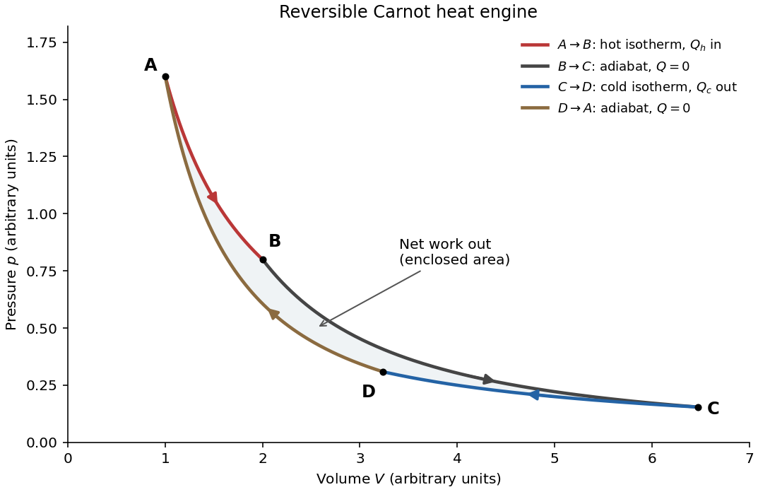
Starting at $A$, perform the following four stages:

The clockwise enclosed area in the pressure-volume diagram is the positive net work per cycle, $W=\oint pdV=Q_h-Q_c$.

For the numbered engine, denote the low and high pressures by $p_1=p_4=p_l$ and $p_2=p_3=p_h$. Let $R_g$ denote the molar gas constant. The ideal gas law makes the constant-pressure branches straight rays in a temperature-volume diagram:The high-pressure ray is steeper. For a constant heat capacity ratio $\gamma$, each reversible ideal-gas adiabat obeysConsequently $1\to 2$ curves upward and left during compression; $2\to 3$ goes upward and right along the steeper ray; $3\to 4$ curves downward and right during expansion; and $4\to 1$ goes downward and left along the shallower ray.

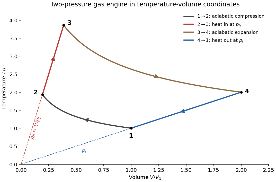
The plot is an original calculation for $\gamma =7/5$, $p_h/p_l=10$ and $V_3/V_2=2$; its state directions follow the original paper. The dashed extensions identify the two constant-pressure rays, not additional stages of the cycle.

A cubic reflecting cavity supports standing waves with positive integer mode indices and wavevector components $k_i=\pi n_i/L$. A cell in mode space has volume $(\pi /L{)}^3$. In the continuum approximation, a spherical shell of radius $k$ and thickness $dk$ has one-eighth of its volume in the positive octant. There are two independent transverse photon polarizations for a generic wavevector. HenceThe photon energy is $ϵ=\hslash \omega =\hslash ck$, so $dk=dϵ/(\hslash c)$. ThereforeThis is the leading bulk density of states, valid when the cavity is large compared with the relevant wavelengths and many modes lie in the counting interval. A finite cavity has a discrete mode spectrum, with boundary corrections beyond this approximation. Modes with vanishing indices require separate boundary counting but do not change the leading $L^3$ term. Here $\hslash$ is the reduced Planck constant, as printed in the original PDF; replacing it by $h$ would introduce an erroneous factor of $(2\pi {)}^3$.

Each independent cavity mode is a quantum harmonic oscillator of angular frequency $\omega$. Its occupation numbers $n=0,1,\dots$ represent the numbers of photons in that mode. At thermal equilibrium, photons can be absorbed and emitted by the walls, so their number is not conserved and the photon chemical potential is zero. The Boltzmann distribution of the oscillator excitations then givesThe expression supplied in the paper is the thermal excitation energy. The oscillator's temperature-independent zero-point energy is excluded from the emitted thermal radiation.

Putting $ϵ=\hslash \omega$ and $dϵ=\hslash d\omega$ into the mode count from (a) gives the number of modes per unit cavity volume:Multiplying by the mean thermal energy in each mode yields Planck's law in the angular-frequency convention:The two photon polarizations are already included in the density of states; no further factor of two is needed. $u(T,\omega )d\omega$ has units $\mathrm{J}{\mathrm{m}}^{-3}$, whereas $u(T,\omega )$ has units $\mathrm{J}\mathrm{s}{\mathrm{m}}^{-3}$.

The equilibrium photon gas is isotropic, so the energy density per unit solid angle in a narrow angular-frequency interval is $u(T,\omega )d\omega /(4\pi )$. For rays making angle $\theta$ with an outward surface normal, a surface element $dA$ is crossed in time $dt$ by rays initially in a volume $cdtdA\cos \theta$. Only the outward hemisphere contributes. ThusThe hemispherical restriction supplies a factor $1/2$ and the directional projection supplies another $1/2$. A small aperture in a cavity therefore emits this spectral power per unit area. A blackbody at the same temperature emits the same amount: otherwise radiation exchange between it and the aperture would violate thermal equilibrium.

Integrating Planck's law over all positive angular frequencies gives the total emitted heat flux densitySet $x=\hslash \omega /(k_{B}T)$. ThenThe remaining integral is independent of temperature, proving $M\propto T^4$. Its value follows by expanding $(e^x-1{)}^{-1}={\sum }_{m=1}^{\infty }{e}^{-mx}$ and integrating termwise:Consequently the Stefan–Boltzmann law isThis is emitted power alone. A body in a radiation environment also absorbs incoming radiation, which must be included when calculating net radiative cooling.

The closed surface integral sums the outward electric flux: $\mathbf{E}$ is the electric field, $d\mathbf{S}$ its outward vector area, $Q$ the total enclosed charge and ${ϵ}_0$ the vacuum permittivity. Gauss's law relates that flux to enclosed charge for any closed surface. High symmetry can make the field's magnitude constant on a suitable Gaussian surface and fix its direction; without symmetry, flux alone does not determine the local field.

For an isolated conducting sphere, charges reside at its surface and the exterior field is radial. ThusThe conductor has zero interior field. Integrating exterior field energy givesLet the initial charge per drop be $q=4\pi {ϵ}_{0}a{V}_1$. After disconnecting the charging supply, charge is conserved. Volume conservation gives final radius $A=2^{1/3}a$, total charge $2q$ andInitial mutual energy is negligible at the stipulated large separation. HenceThe electrostatic energy increase on equal-drop coalescence is positive. It can be supplied by the decrease in surface energy during coalescence and/or by external mechanical work bringing like charges together. Remaining energy can become motion and heat. If the charge is too large, surface-energy release alone need not suffice to make merging spontaneous; conservation does not assert that it will. Keeping the drops connected to a voltage supply would instead be a different charge-balance problem.

In vacuum the electric and magnetic field energy densities areFor example, charging a capacitor requires $U={\int }_0^Q(q/C)dq=Q^2/(2C)=C{V}^2/2$. A parallel-plate capacitor with $C={ϵ}_{0}A/d$ and $E=V/d$ then gives $U={ϵ}_0{E}^{2}Ad/2$, identifying the electric field energy density. Similarly an inductor stores $L{I}^2/2$; applying this to a long solenoid yields $B^2/(2{\mu }_0)$ times its interior volume.

Electromagnetic energy is transported by the Poynting vector $\mathbf{S}=\mathbf{E}\times \mathbf{B}/{\mu }_0$. Poynting's theorem,expresses local energy conservation and transfer to matter. In a vacuum plane wave $E=cB$, so the two energy densities are equal and the energy flux has magnitude $c(u_E+u_B)$. For nondispersive linear media the corresponding reversible expressions are $\mathbf{E}\cdot \mathbf{D}/2$ and $\mathbf{B}\cdot \mathbf{H}/2$; they must not be applied unchanged to arbitrary dispersive or hysteretic materials.

An impulse is $\mathbf{J}=\int \mathbf{F}dt$, giving $\Delta \mathbf{P}=\mathbf{J}$. For a short localized impulse at displacement $\mathbf{r}$ from the centre of mass, the angular impulse is $\Delta {\mathbf{L}}_{\mathrm{CM}}=\mathbf{r}\times \mathbf{J}$; for a changing lever arm use its instantaneous value inside the integral. For a uniform solid sphere with volume density ${\rho }_V$, direct integration about the $z$ axis givesTake forward translation $u$ and forward-rolling clockwise spin $\Omega$ as positive. Neglect the table's tangential impulse during the much shorter cue impact. Immediately afterwards,The bottom contact point has slip velocity $s_0=u_0-a{\Omega }_0$. The cue height for immediate rolling is therefore $d=2a/5$.

For the impulse-driven slipping-to-rolling transition of a sphere at an arbitrary admissible impact height, let $J_f$ be the signed friction impulse accumulated before slipping ends. Translation and spin then obey $u_f=u_0+J_f/M$ and ${\Omega }_f={\Omega }_0-a{J}_f/I$. Impose $u_f=a{\Omega }_f$ and eliminate $J_f$:This expression handles both sliding directions. If $d<2a/5$, the contact point slips forward and friction slows the centre; if $d>2a/5$, excess spin makes it slip backward and friction accelerates the centre. friction still dissipates total mechanical energy. For ${\mu }_d>0$, $\dot{s}=-(7/2){\mu }_{d}g\mathrm{sgn}s$, so the slipping time is $2|s_0|/(7{\mu }_{d}g)$. Its duration depends on friction, while the final speed does not. With zero friction no slipping-to-rolling transition occurs unless rolling was present from the outset.

Let the cylinder length be $\ell =0.020\mathrm{m}$, cross-sectional area $A$, and the fluid mass density ${\rho }_f$. At floating equilibrium, Archimedes' principle givesFor a small downward displacement $z$ from this equilibrium, the displaced fluid volume increases by $Az$. The additional upward buoyant force is ${\rho }_{f}gAz$, and Newton's second law becomesThis is simple harmonic motion, with angular frequency $\omega =\sqrt{2g/\ell }$ and oscillation periodThe result for vertical oscillations of a floating cylinder is independent of its cross-sectional area and fluid mass density because those quantities cancel using the known immersion fraction. It neglects drag, surface effects and the extra fluid inertia from the motion; the cylinder must remain partly immersed throughout the small motion.

With microstate energies held fixed when differentiating,Since $d\beta /dT=-1/(k_B{T}^2)$,The canonical ensemble fixes volume and particle number, and any other external Hamiltonian parameters. Thus the derivative is $C_V$; pressure-fixed fluctuations would naturally involve enthalpy in a different ensemble.

The translational and two-level energy variance follows because translation and internal states factorize for this dilute classical gas:Differentiating twice yieldsThe terms are independent translational and two-level binomial variances. At $k_{B}T\ll ϵ$, excitation freezes out exponentially and translation dominates. At $k_{B}T\gg ϵ$, the internal variance tends to $N{ϵ}^2/4$ while the translational variance grows as $T^2$; the internal heat capacity consequently tends to zero. Fractional total-energy fluctuations are of order $N^{-1/2}$ for large $N$. The low-temperature statement presumes translation is still nondegenerate; at strictly zero temperature the classical-gas model fails.

Let $a$ be the cube's side and $z$ a small upward displacement. Its displaced water volume decreases by $a^{2}z$, so the change in buoyancy is $-{\rho }_{w}g{a}^{2}z$. With cube mass $m=0.9{\rho }_w{a}^3$,The displacement must be small enough that the upper face remains above water and the bottom remains submerged. This buoyancy estimate neglects fluid added mass, damping and melting.

The quasistatic pressure-volume work done on the body is $\delta W=-PdV$. If its volume remains constant throughout the process, every $dV$ vanishes, so the work is zero. Equal initial and final volumes alone would not suffice: an expansion and compression cycle can have nonzero work. Other work modes are excluded by this simple elastic-volume model.

Within the stated small-volume-change approximation, treat $V,{\kappa }_T,\alpha$ in the differential constitutive law as constants. ThenPath (a) first changes temperature at pressure $P_1$, then changes pressure at fixed temperature $T_2$. The two contributions are $-V_1\alpha P_1(T_2-T_1)$ and $V_1{\kappa }_T(P_2^2-P_1^2)/2$. ThereforeWork is path dependent even though the endpoints and approximate total volume change are the same.

Path (b) changes pressure before temperature. Its pressure integral is unchanged, but the thermal expansion occurs at $P_2$:Along the straight path (c), $P=P_1+(P_2-P_1)(T-T_1)/(T_2-T_1)$. Thus ${\int }_{T_1}^{T_2}PdT=(P_1+P_2)(T_2-T_1)/2$, while $\int PdP$ depends only on the pressure endpoints. ConsequentlyThis pressure-temperature path-work identity is a consequence of the linearized volume law and the straight interpolation. It need not hold for strongly varying compressibility or expansion coefficient.

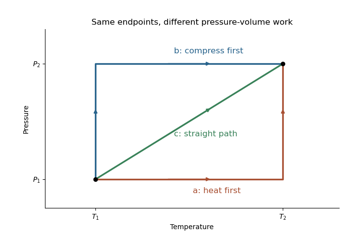
Illustration TODO. The source's two-volume circulation sketch on page 4 is unavailable. Its exact arrows and layout cannot be recovered. The surviving flow law, salinity/temperature definitions and printed steady polynomial allow the calculation below under an explicit freshwater sign convention; no unavailable diagram values are invented.

Use $\Delta T=T_2-T_1>0$, $\Delta S=S_2-S_1$, and let positive $q$ be the thermally driven state with cold box 1 denser than warm box 2. Take positive $F$ to freshen box 1, represented in a fixed-volume salt budget by an equivalent salt removal $F{S}_1$ from that box and addition to the other reservoir. This is the freshwater convention compatible with the printed $+BF$ and positive $B$. It can represent a compensating saline volume transfer or the usual virtual-salt-flux approximation. The exact pipe assignment is not claimed to have been read from the missing illustration.

Exchange in either circulation direction reduces a salinity difference at rate proportional to $|q|\Delta S$. Steady salt balance therefore givesThe supplied linear equation of state givesEliminating $\Delta S$ yields the two-box overturning model equationHere $A$ and $B$ both have transport units when $q,F,k$ do, while $\alpha \Delta T$ and $\beta S_1$ are dimensionless. Although the source calls $q$ a mass flow, its stated Sverdrup units are volume per time; the common reference density cancels in the Boussinesq salt/volume approximation. At $F>0$, $q=0$ cannot be a finite-salinity steady state in this model. At $F=0$, zero flow needs separate treatment instead of division by $|q|$.

The circulation weakens when freshwater freshens the cold reservoir, and the weaker circulation removes the resulting salinity contrast less effectively. This salt-advection feedback is the mechanism behind multiple steady states, not an additional externally imposed switch.

Cooling makes the oceanic lithosphere denser and contracts it; isostatic adjustment therefore lowers the seafloor. The cooling layer includes substantial mantle, not just the approximately fixed-thickness igneous oceanic crust.

New plate near a spreading ridge is hot and relatively buoyant. As it moves away, conductive cooling penetrates more deeply, and material formerly in the hot asthenosphere becomes part of the colder thermal boundary layer. To first order,where $\alpha$ is the volumetric thermal expansion coefficient, ${\rho }_m$ a reference mantle density, $T_m$ the hot reference temperature, and $t$ plate age. A positive depth-integrated density anomaly makes the column negatively buoyant relative to the ridge column. Isostasy is restored by downward displacement and mantle redistribution; cold rock also occupies less volume.

At a fixed sufficiently deep datum, deepening the seafloor by $\Delta d$ removes an equivalent thickness of rock from the column and replaces it with less dense seawater. In the usual constant-property approximation this giveswhere ${\rho }_w$ is seawater density and $z_c$ lies below the relevant thermal anomaly. This explains why contraction alone and water-loaded seafloor subsidence are not identical numerical quantities.

For a half-space cooling model,so integration yieldsHere $\kappa$ is thermal diffusivity and $z$ is measured downward from the surface of the thermal model. The leading oceanic thermal subsidence is proportional to $\sqrt{t}$. A finite oceanic plate cooling model limits this growth at old ages. Sediment loading, dynamic topography, anomalous crust thickness and hydrothermal heat transport can produce departures from the simple relation.^[ref]

Specify what “onset” means. I would distinguish the first local, perhaps short-lived subduction event from persistent, self-sustaining recycling in a connected global network of tectonic plates. Modern plate tectonics combines relatively rigid moving lithosphere, localized boundary deformation, seafloor spreading and sustained convergence. A sinking drip or a single imposed descending sheet is not sufficient evidence of that global regime. Different processes may become established at different times, so a transition interval may be a better hypothesis than an instantaneous worldwide switch.

Construct competing physical models. Solve conservation of mass, momentum and energy for evolving mantle convection and lithosphere, including temperature- and stress-dependent rheology, brittle yielding, plastic deformation, melting, compositional buoyancy and relevant phase changes. Use geodynamic modelling to compare a stagnant lid, episodic overturn, drip-dominated recycling and a sustained mobile lid. In a simplified incompressible creeping-flow framework,Here $\mathbf{u}$ is velocity, $p$ pressure, $\eta$ effective viscosity, $\dot{\mathbf{ϵ}}$ the strain-rate tensor, $\rho$ density, $\mathbf{g}$ gravitational acceleration, $c_p$ specific heat capacity, $k$ thermal conductivity, $H$ radiogenic power per unit mass, and $\Phi$ dissipative heating per unit volume. These equations are a framework: compressibility, latent heat and chemical transport may require additional terms. A simple yield stress law ${\tau }_y=C+\mu (\rho gz-P_f)$ represents cohesion $C$, friction coefficient $\mu$ and pore pressure $P_f$, illustrating why hydration and interface weakening can change the outcome.

Vary the early-planet controls rather than assuming the answer. Explore plausible initial mantle potential temperature, radiogenic heating, crust thickness and composition, water inventory, grain-size evolution, surface temperature, and boundary strength. Hotter mantle lowers viscosity but can produce thicker buoyant basaltic crust; it does not automatically make sustained subduction easier. A cold strong plate can transmit slab pull yet resist bending and initiation. Water weakening of rocks, melt-induced weakening, inherited faults and mechanically weak sediments can change this balance. Test proposed triggers such as mantle plume impingement or gravitational instability without presupposing an established global plate-force system.

Useful diagnostics include the Rayleigh number,with thermal expansion coefficient $\alpha$, layer thickness $D$, thermal diffusivity $\kappa$ and temperature contrast $\Delta T$, together with surface mobility, the localization of deformation, plate longevity, melt production and material recycling. A large Rayleigh number establishes vigorous convection under suitable conditions, not necessarily a mobile lid. A convincing model should sustain one-sided subduction, connected boundary evolution and seafloor spreading after any artificial trigger is removed. Compare initiation thresholds with continuation thresholds: hysteresis can allow an established regime to persist under conditions in which it would not spontaneously start.

As an example of the type of experiment, three-dimensional models have tested mantle plume-induced subduction initiation, finding sensitivity to plate buoyancy, magmatic weakening and hydration of the interface. The scientific use of such results here is to identify a feasible mechanism and its predicted signatures, not to adopt their success as a direct measurement of an ancient onset date.^[ref]

Connect a model regime to a date through independent evidence. Couple the experiments to candidate planetary cooling histories, then predict observable pressure-temperature-time paths, magmatic compositions, deformation patterns and recycling rates for each regime. If independently dated rocks constrain a thermal or compositional state, ask which regimes can reproduce that state and the observed geological associations. Repeat over uncertain initial conditions and constitutive parameters, check numerical resolution, and compare two- and three-dimensional results where geometry matters. Models that prescribe a descending slab, fix plate velocity, or insert a weak boundary may be excellent forward models of a working subduction zone but do not demonstrate spontaneous initiation.

The result is a conditional statement: persistent plate tectonics is physically feasible under a range of conditions, and dated geological observations may favor that range at a particular time. Uncertain cooling histories, several feasible regimes and uncertain rheology prevent numerical feasibility alone from dating onset. The strongest constraint comes when the same parameter range explains multiple independently dated observations and alternative regimes fail those tests.

For a normal constrained extremal, introduce a constant Lagrange multiplier and use $L=F-\lambda G$. The Euler-Lagrange equation isWhen both integrands have no explicit $x$ dependence, the Beltrami identity gives $L-y^{\prime }{L}_{y^{\prime }}=\text{constant}$, as follows by differentiating this expression and using the Euler-Lagrange equation.

Parametrize the surface by $(f(z)\cos \theta ,f(z)\sin \theta ,z)$. The cross product of its two coordinate tangents has magnitude $f\sqrt{1+(f^{\prime }{)}^2}$, so integration in $\theta$ gives $A=2\pi {\int }_a^{b}f\sqrt{1+(f^{\prime }{)}^2}dz$. Integrating the cross-sectional disk areas gives $V=\pi {\int }_a^b{f}^{2}dz$.

Dividing the augmented functional $A-\lambda V$ by $\pi$, useThe Euler-Lagrange equation isThe Beltrami identity becomes $2f/\sqrt{1+(f^{\prime }{)}^2}-\lambda f^2=C$. At an endpoint $f\to 0$, the absolute value of the first term is at most $2f$, so $C=0$, even if the profile has an infinite endpoint slope. For a nondegenerate regular closed surface take $f>0$ on $(a,b)$. Then $\lambda >0$, and, with $R=2/\lambda$,Combining this identity with the Euler-Lagrange equation yields $f^{\prime \prime }=-R^2/f^3$. Consequently $(f^2{)}^{\prime \prime }=2((f^{\prime }{)}^2+f{f}^{\prime \prime })=-2$. The two zero endpoint values uniquely determineThe positive radius profile is therefore a semicircle and generates a sphere, centred at height $(a+b)/2$, with radius $R=(b-a)/2$. In particularThe graph is smooth in the interior; its vertical slopes at the two poles are compatible with a smooth spherical surface. Its volume is $4\pi R^3/3$, the volume associated with this stationary candidate.

For minimality, the three-dimensional isoperimetric inequality says that every closed surface enclosing volume $V$ has $A^3\ge 36\pi V^2$, with equality for a sphere. The displayed extremal attains equality, proving that it minimizes area at its fixed enclosed volume. The uniqueness above concerns the regular connected positive profile with the two stated endpoint heights.