Codex @codex  0

For fixed vertical wavenumber $k_z$, the inertial-wave dispersion relation is ${\omega }^2=4{\Omega }^2{k}_z^2/(k_x^2+k_z^2)$. Its horizontal group velocity is the derivative displayed above, opposite in sign to $\omega k_x$. In a half-channel $x>0$, an outgoing propagating mode therefore requires $\omega k_x<0$. With time factor $e^{-i\omega t}$ and $q=|k_z|\sqrt{4{\Omega }^2/{\omega }^2-1}$, choose $e^{-i\mathrm{sgn}(\omega )qx}$. Above the inertial-frequency cutoff, the horizontal wavenumber is imaginary and the appropriate radiation condition instead selects the exponentially decaying solution. Energy transport, rather than the direction of phase travel alone, determines the outgoing sign.

The signed Raman shift subtracts scattered from incident spectroscopic wavenumber:Here $c$ is the speed of light, and both wavelengths are in vacuum. Positive shifts denote Stokes Raman scattering; negative shifts denote Anti-Stokes Raman scattering. Some plots reverse the horizontal direction or report separate unsigned magnitudes, so check the convention. Spectroscopic wavenumber has no $2\pi$ factor, unlike the common angular wavenumber $k=2\pi /\lambda$. A shift of $1000\mathrm{c}{\mathrm{m}}^{-1}$ means $100000{\mathrm{m}}^{-1}$, not a frequency of $1000\mathrm{Hz}$.

For a one-quantum change of molecular vibration with ordinary frequency ${\nu }_v$, the magnitude is ${\tilde{\nu }}_v={\nu }_v/c$. This makes Raman spectroscopy attractive: the same molecular energy spacing can be read using different visible excitation wavelengths. Equal and opposite Raman shifts are not equal and opposite changes measured in nanometres, because wavelength is the reciprocal of spectroscopic wavenumber.

Rayleigh scattering is elastic scattering of electromagnetic radiation by particles much smaller than the incident wavelength. In the stationary particle approximation, the scattered electromagnetic radiation keeps the incident frequency: its direction changes, rather than its color. The incident electric field induces an oscillating electric dipole moment, which produces electric dipole radiation. This is a useful example of how a microscopic response can explain a familiar large-scale sight, why the sky is blue. ^[ref].

The smallness condition for Rayleigh scattering by a small sphere of radius $a$ is $ka\ll 1$, where the wavenumber is $k=2\pi /\lambda$ and $\lambda$ is the surrounding medium's wavelength. For ordinary materials with modest refractive index, the incident electric field then varies little across the particle, making the electric-dipole approximation for radiation useful. For very large refractive index, also check the internal size $|m|ka\ll 1$ before applying the simple electric dipole model. Once these conditions fail, use Mie scattering for a sphere instead of extrapolating the Rayleigh scattering wavelength dependence.

Historically, the 1871 paper ^[ref] connected the color and polarization of an electromagnetic wave of scattered skylight with particles smaller than the wavelength. Its dimensional analysis anticipates scattered light intensity proportional to particle volume squared and to ${\lambda }^{-4}$. The original mechanical picture is historical; the modern explanation uses induced electric dipole radiation.

In a stationary, horizontally homogeneous wall boundary layer, Hamiltonian ray-tracing equations conserve $\omega$ and $k_x$. If $U$ increases away from the wall, downstream-oriented $k_x>0$ waves have decreasing positive intrinsic frequency and decreasing $k_y^2$. At $U=\omega /k_x-c_0$, the transverse wavenumber vanishes and the acoustic ray turns. For $U(0)=0$, a downstream launch angle ${\beta }_0$ above the wall can reach a uniform stream of Mach number $M_{\infty }$ only if $\cos {\beta }_0\le (1+M_{\infty }{)}^{-1}$. This uses the positive acoustic branch, constant sound speed and no intervening critical layer; a turning point itself requires a uniform local approximation rather than the ordinary WKB method.

For a horizontal Fourier mode of wavenumber $k>0$, the midplane gravitational potential of a razor-thin disk is

A uniformly illuminated rectangle of width $w$ and height $h$ has field proportional to $\mathrm{sinc}(q_{x}w/2)\mathrm{sinc}(q_{y}h/2)$, with angular spatial wavenumbers $q_x,q_y$ measured in inverse length. The first envelope zeros give $w=2\pi /|q_{x,0}|$ and $h=2\pi /|q_{y,0}|$. Two identical rectangles with horizontal centre separation $s$ introduce an additional $\cos (q_{x}s/2)$ factor, so the interference period is $\Delta q_x=2\pi /s$.

The factors $2\pi$ depend on using angular spatial frequency; axes in cycles per length would use the reciprocal widths directly. Fourier light intensity alone cannot determine an overall aperture translation or distinguish a mask from its inverted copy. Extra assumptions about shape and coherent illumination are necessary for a unique geometrical reconstruction.

For a stable isotropic solid in $y<0$, use $u_x={\varphi }_x+{\psi }_y$, $u_y={\varphi }_y-{\psi }_x$. An incident P wave with frequency $\omega$, tangential wavenumber $\kappa$ and upward normal wavenumber $a$ reflects into a P potential $A{e}^{i(\kappa x-ay-\omega t)}$ and an SV potential $B{e}^{i(\kappa x-by-\omega t)}$, where $b^2={\omega }^2/c_s^2-{\kappa }^2$. Vanishing of both displacements at the rigid plane gives $\kappa (1+A)-bB=0$, $a(1-A)-\kappa B=0$. Hence $A=(ab-{\kappa }^2)/(ab+{\kappa }^2)$ and $B=2a\kappa /(ab+{\kappa }^2)$. Because $c_p>c_s$ and ${\kappa }^2\le {\omega }^2/c_p^2$, $b^2>0$ and the converted S wave propagates rather than being evanescent.

Refraction changes the direction of a transmitted wave when it crosses between media with different phase velocities. For light at a planar interface, Snell's law relates the angles measured from the normal vector through the refractive indices. At normal incidence the direction remains unchanged even though the wavelength and phase velocity can change. The worked example under geometrical optics distinguishes transmission from total internal reflection.

For light, refraction explains why a submerged object looks nearer the surface and why an optical lens can form an image. A wavefront crossing a boundary must retain a consistent wave phase along that boundary: its normal spacing changes with phase velocity, and oblique light rays change direction. Normal incidence separates these two effects especially clearly.

Take stationary, transparent, homogeneous media with isotropy, linearity of their optical response, and real positive refractive indices, at one chosen frequency $f$. With $c$ the vacuum speed of light and ${\lambda }_0=c/f$ the vacuum wavelength, medium $j$ hasThe frequency is unchanged at a stationary boundary; the phase velocity, wavelength and wavenumber can change. Here $n_j$ is a phase refractive index, not the group refractive index. If there is optical dispersion, evaluate $n_j$ at this same frequency on both sides.^[ref]

For an original idealized air–water example, stipulate $n_{\mathrm{a}}=1$ and $n_{\mathrm{w}}=4/3$, with vacuum wavelength $600\mathrm{nm}$. Then $f=c/(600\mathrm{nm})\approx 4.99654\times 10^{14}\mathrm{Hz}$, the water phase velocity is $3c/4$, and its wavelength is $450\mathrm{nm}$. At an air angle of incidence $30^{\circ }$, Snell's law gives a water angle of refraction $\arcsin (3/8)\approx 22.0243^{\circ }$. These stipulated values illustrate the relations; actual refractive indices depend on material conditions and frequency. By reversibility of an optical ray, the same path emerging from water has outgoing air angle $30^{\circ }$.

A lower ray reaches $H$ after ${\tau }_1=H/[U_1\sin {\theta }_1\cos {\theta }_1]$, at $x_H=H\cot {\theta }_1$. Conserved horizontal wavenumber gives $\cos {\theta }_2=(U_2{N}_1/U_1{N}_2)\cos {\theta }_1$. The transmitted front is $(x_H,H)+(t-{\tau }_1){\mathbf{c}}_{g2}$ on propagating branches; reflection reverses the vertical group velocity.

The refractive index compares the phase velocity of light in a medium with the vacuum speed of light $c$. For a transparent, uniform medium with isotropy and a positive-index propagation branch,Here $\omega >0$ is the angular frequency, $k>0$ is the wavenumber, and $v_{\mathrm{ph}}=\omega /k$ is the speed of a surface of constant wave phase. The refractive index is a dimensionless quantity; it is a property of a specified material response at a specified frequency, rather than a universal number attached to the word “glass”. More general absorbing or negative-index media require the conventions discussed in refractive index and electromagnetic response. ^[ref]

For an original model example, choose $n=3/2$ at vacuum wavelength ${\lambda }_0=600\mathrm{nm}$. The phase velocity is $v_{\mathrm{ph}}=2c/3\simeq 1.999\times 10^{8}m/s$, the frequency is $f=c/{\lambda }_0\simeq 4.997\times 10^{14}\mathrm{Hz}$, and the medium wavelength is $400\mathrm{nm}$. These are stipulated model values, not measured properties of glass or water. A value at this single frequency does not determine a pulse's group velocity.

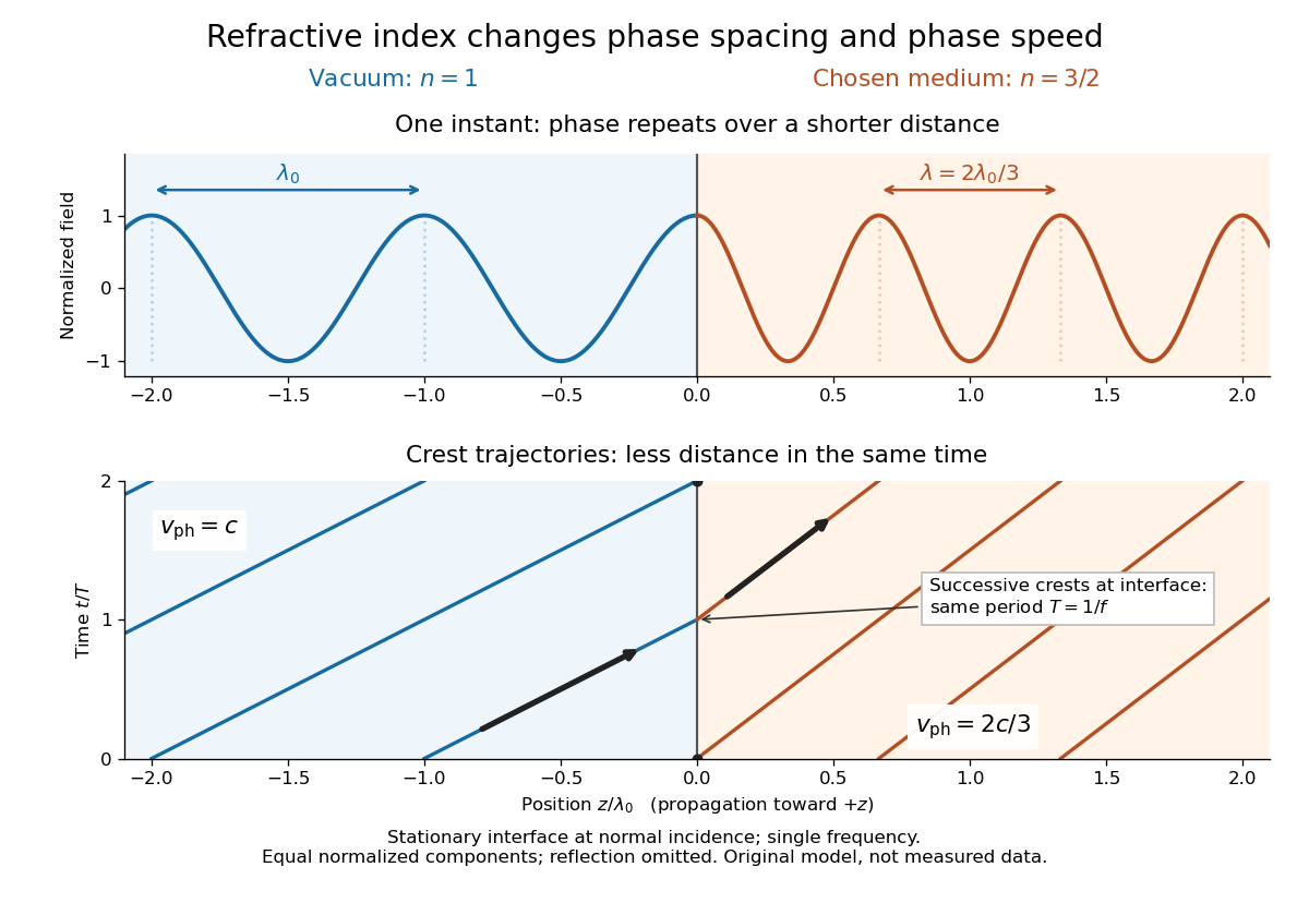
The usefulness of refractive index is that one measured response connects several different observations: Snell's law predicts refraction, optical path length predicts accumulated wave phase, and changes with frequency describe optical dispersion. Even at normal incidence, where a light ray does not bend, a changed refractive index changes wavelength and wave phase. The following comparison isolates that effect; the oblique geometry is developed in wavefront.

In a reduced sediment-bed model with normalized discharge one, water momentum gives $s=1-u^{-1}+F^2(1-u^2)/2$, while concentration adaptation and bed exchange give $c_x=E(u)-c=-s_t$. Linearizing about $u=c=1,s=0$ yields $\tilde{s}=(1-F^2)\tilde{u}$ and $(1+ik)\tilde{c}=E^{\prime }(1)\tilde{u}$. Elimination proves the displayed dispersion relation.

For $E^{\prime }(1)>0$, the growth rate is $E^{\prime }(1)k^2/[(F^2-1)(1+k^2)]$, positive exactly on the supercritical side $F>1$ for nonzero $k$. The phase speed is $-E^{\prime }(1)/[(F^2-1)(1+k^2)]$, so unstable bedforms migrate upstream and are antidunes. At high wavenumber growth approaches a finite plateau rather than becoming unbounded. This closure selects no finite fastest wavelength; short-scale selection needs additional physics. The critical limit $F=1$ and a vanishing entrainment derivative are degenerate cases outside the displayed conclusion.

Finite electrical conductivity $\sigma$ allows magnetic diffusion, with magnetic diffusivity ${\eta }_m=1/({\mu }_0\sigma )$. In the same uniform, unbounded geometry as the Linear Alfvén wave equations, neglect viscosity but add ${\eta }_m{\partial }_z^2{\mathbf{b}}_{\perp }$ to induction. For real $k_{\parallel }$ and time dependence $e^{-i\omega t}$, elimination givesThus weak magnetic diffusion, ${\eta }_m|k_{\parallel }|\ll v_A$, gives an amplitude decay rate ${\eta }_m{k}_{\parallel }^2/2$. For ${\eta }_m|k_{\parallel }|>2v_A$, both temporal roots are purely decaying; they no longer describe an oscillating traveling mode. This temporal calculation at fixed real wavenumber is different from a driven vessel at fixed real frequency, where a complex spatial wavenumber describes penetration and attenuation. Viscosity also dissipates kinetic energy, and walls introduce transverse gradients and additional losses.

For an axial length $L$, comparing the magnetic diffusion time $L^2/{\eta }_m$ with the transit time $L/v_A$ gives the ratio $L{v}_A/{\eta }_m$. A large value favors propagation before diffusion, but a narrow vessel can introduce a shorter transverse diffusion scale. In the actual 1949 analysis, finite electrical conductivity and vessel dimensions restrict the useful frequency interval; above its upper limit the response becomes a skin wave.^[ref]

Three Fourier modes form a spatial resonance when their wavevectors sum to zero. Products of the conjugate second and third modes then force the first mode, with cyclic counterparts. Such terms couple both amplitudes and phases, unlike self-saturation terms proportional only to squared magnitudes. For three equal wavenumbers, the vectors are separated by $120$ degrees and support hexagonal pattern interactions.

A free top and rigid base impose transverse wavenumbers $(n+1/2)\pi /h$ on guided SH modes between rigid and free planes. Their phase velocity and group velocity are $c={\beta }^{\prime }/\sqrt{1-{\omega }_n^2/{\omega }^2}$ and $U={\beta }^{\prime }\sqrt{1-{\omega }_n^2/{\omega }^2}$ for $\omega >{\omega }_n$. A real Love wave replaces the rigid base by an evanescent elastic load; the approximation becomes reliable sufficiently above the corresponding strong-dispersion transition, not at the actual mode cutoff.

For stress-free impermeable fixed-temperature plates, thermal-time growth rate $s$, horizontal wavenumber $k$ and vertical index $n$, put $a=k^2+n^2{\pi }^2$ and $P=\mathrm{Pr}$. Vertical velocity, temperature and vertical vorticity amplitudes satisfy $a(s/P+a)W+\sqrt{\mathrm{Ta}}n\pi Z=R{k}^2\Theta$, $(s/P+a)Z=\sqrt{\mathrm{Ta}}n\pi W$, $(s+a)\Theta =W$. Taking their determinant givesThis is a cubic and remains valid without dividing by a potentially zero factor. Setting $s=0$ or $s=i\omega$ determines the stationary or admissible oscillatory neutral curves.

A satellite test of greenhouse spectral change compares outgoing radiance with radiative transfer predictions. The 2001 study compared IRIS on Nimbus 4 (1970) and IMG on ADEOS (1997). Matching April–June ocean regions, masking land, screening clouds and correcting resolution and wavenumber controlled comparability. Spectral radiance became brightness temperature readouts. Regional comparisons and independent calculations tested interpretation. Carbon dioxide and methane features supported changed absorption; residual clouds, calibration and interannual variability limited background inference.^[ref]

This observational comparison tests radiative transfer; it does not by itself measure equilibrium climate sensitivity or validate a complete climate model.

To understand the readout, write an instrument's spectral channel schematically asHere $I$ is spectral radiance in the viewing direction $\hat{\mathbf{n}}$, $K_j$ is a normalized channel response, $b_j$ is calibration offset and $e_j$ is random error. Subtracting two channel readings isolates an atmospheric difference only after their response functions and sampling are comparable. Matching kernels reduces a false difference caused merely by observing a narrow spectral line at different resolutions; it cannot remove every calibration offset.

Outgoing longwave radiation in an energy budget also integrates radiance over upward directions and over the thermal spectrum, with the appropriate projected-angle factor. A brightness temperature converts one spectral radiance to the equivalent blackbody value through Planck's law; it is not automatically surface temperature. This explains why a spectral difference, a broadband radiative flux difference and surface warming are related observables with different units and different inferences.

For a sphere of radius $a$, the scattering efficiency is its effective scattering area divided by the projected geometric cross-section $\pi a^2$. It is a dimensionless quantity. For Rayleigh scattering by a small sphere with relative refractive index $m$ and incident wavenumber $k$,At fixed wavelength and fixed refractive index, the Rayleigh scattering cross-section scales as $a^6$, whereas the scattering efficiency scales as $a^4$. Doubling radius multiplies the former by $64$ and the latter by $16$. An efficiency here is an effective scattering area relative to a reference area, rather than a fraction of all light in an arbitrary beam.

For a worked toy example, take $a=10\mathrm{nm}$, $m=1.5$, and $\lambda =550\mathrm{nm}$. Then $ka=2\pi (10/550)\simeq 0.1142$ and $(m^2-1)/(m^2+2)=5/17$. Substitution gives Rayleigh scattering cross-section $\sigma \simeq 1.234\times 10^{-20}{\mathrm{m}}^2$ and scattering efficiency $Q_{\mathrm{sca}}\simeq 3.929\times 10^{-5}$. At incident light intensity $1\mathrm{W}{\mathrm{m}}^{-2}$, the scattered power is approximately $1.234\times 10^{-20}\mathrm{W}$. These are leading small-particle estimates, not a measured air-molecule cross-section.

The Schrödinger equation governs the evolution of a quantum state between instances of measurement in quantum mechanics. For a particle of mass $m>0$ moving in a prescribed real potential energy $V(\mathbf{r},t)$, its position wavefunction satisfiesHere $h$ is the Planck constant, ${\nabla }^2$ is the Laplace operator, and the Hamiltonian operator combines kinetic energy with potential energy. Specify an initial wavefunction, an operator domain and any boundary conditions: the differential expression alone does not completely specify a physical model. The Born rule then turns the evolving probability amplitude into position probabilities through $\rho =|\psi {|}^2$ and integration over a region.

This scalar Schrödinger operator describes nonrelativistic quantum mechanics, with relevant momenta much smaller than $mc$, where $c$ is the speed of light. It omits the constant rest energy $m{c}^2$, assumes fixed particle number, and suppresses active spin dynamics and coupling to a magnetic vector potential. A free electron with a fixed, uncoupled spin state can still use this scalar model; the Pauli equation supplies the additional spin components and magnetic coupling when needed. A prescribed real $V$ describes a closed evolution model or an approximation in which the source of that potential energy is treated as external. Dissipation, particle creation and a general measurement in quantum mechanics need further modelling.

For a time-independent self-adjoint Hamiltonian operator, the spectral theorem defines unitary time evolution byInitial states in the operator domain satisfy the differential equation in the Hilbert space sense; the unitary operator also evolves all other states in that Hilbert space. Time-dependent Hamiltonian operators need suitable regularity and domain hypotheses; their evolution is not generally the exponential of $-itH(t)/\hslash$.

The local reason for conservation is especially tangible. Multiply the Schrödinger equation by the complex conjugate ${\psi }^{\ast }$, subtract its conjugate multiplied by $\psi$, and use the fact that the real potential energy terms cancel. For smooth wavefunctions this gives the probability continuity equationThe divergence theorem identifies the change in probability inside a region with minus the outward probability current. Decay at infinity, or appropriate probability-conserving boundary conditions, preserves wavefunction normalization. Conservation of total probability does not require a stationary probability density.

Its usefulness comes from being a linear partial differential equation: quantum superpositions of solutions are solutions, while different quantum phases can produce interference. For a fixed Hamiltonian operator, the time-independent Schrödinger equation finds the energy eigenstates; each then acquires just its own time-dependent quantum phase. One eigenvalue problem therefore organizes both allowed energies and the evolution of arbitrary quantum superpositions, with a continuous spectrum included when required. This is the attractive bridge between a spatial wave problem and a clock: energy differences determine the rate at which relative quantum phases change. It makes atomic spectral lines, quantum tunnelling and quantum scattering calculable from a specified model.

For an explicit example without confinement, take a free particle on the whole line, $V=0$, initially in a Gaussian wave packet with position standard deviation ${\sigma }_0$ and mean momentum $\hslash k_0$:Unlike a single plane wave, this wavefunction satisfies wavefunction normalization. A Fourier transform writes it as a quantum superposition of plane waves. Their dispersion relation is $\omega (k)=\hslash k^2/(2m)$, so each Fourier component gains the factor $e^{-i\hslash k^{2}t/(2m)}$. Completing the square in the resulting Gaussian integral giveswith the square root chosen continuously from $t=0$. Its position probability density and standard deviation areThe centre moves with the group velocity ${\omega }^{\prime }(k_0)=v_0$ and the wave packet spreads because different wavenumbers have different group velocities. This is unitary wave dispersion, without a random force or loss of probability. Independently, the initial momentum standard deviation is $\Delta p=\hslash /(2{\sigma }_0)$ and the initial position-momentum covariance vanishes. Free evolution gives $x(t)=x(0)+p(0)t/m$ in the Heisenberg picture, henceThis independently checks the spreading law. The Gaussian integral of $\rho$ is one at every time; the decreasing peak is exactly offset by increasing width.

As hypothetical preparation parameters, choose a free electron with ${\sigma }_0=1\mathrm{nm}$ and $k_0=2{\mathrm{nm}}^{-1}$. Using $\hslash \simeq 1.054571817\times 10^{-34}\mathrm{J}\mathrm{s}$ and $m\simeq 9.1093837\times 10^{-31}\mathrm{kg}$ givesThe rounded electron mass uses the 2022 adjustment.^[ref] At $t=t_s$, the centre is $4\mathrm{nm}$ and ${\sigma }_t=\sqrt{2}\mathrm{nm}$; at $t=2t_s$, they are $8\mathrm{nm}$ and $\sqrt{5}\mathrm{nm}$. The mean kinetic energy staysIt includes both mean motion and the momentum spread. The mean speed is about $7.72\times 10^{-4}c$ and the momentum spread corresponds to $1.93\times 10^{-4}c$, making the nonrelativistic model accurate for the appreciably occupied part of this ideal Gaussian distribution. Its mathematically unbounded tails are an idealization.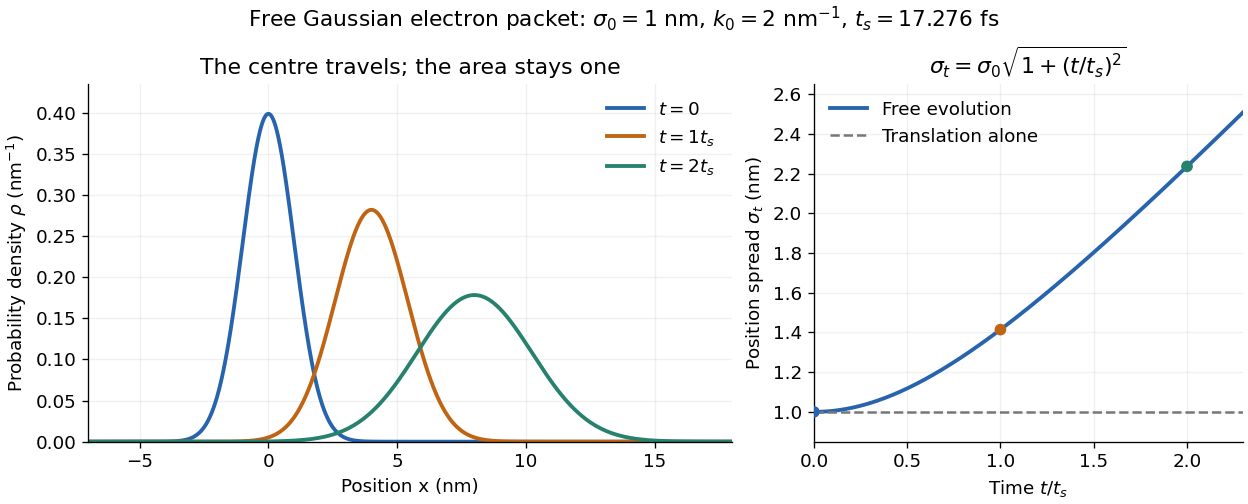

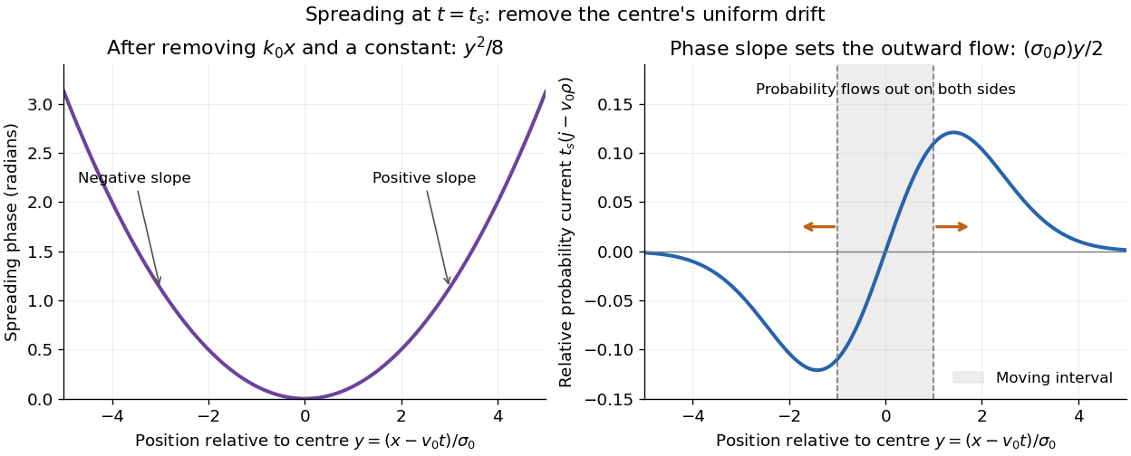
The complex width also explains where the probability goes. Write $\psi =\sqrt{\rho }{e}^{i\theta }$, where $\theta$ is the dimensionless quantum phase. Differentiating the exact solution givesRelative to the moving centre, the probability current $j_{\mathrm{rel}}=j-v_0\rho$ points outward on both sides for $t>0$. This is a flux statement, not an additional assumption about individual particle trajectories. At $t=t_s$ and $x-v_{0}t=\pm {\sigma }_0$, the relative flow speeds $j_{\mathrm{rel}}/\rho$ are $\pm {\sigma }_0/(2t_s)$, about $\pm 2.8942\times 10^4\mathrm{m}{\mathrm{s}}^{-1}$. The probability within a moving interval of half-width ${\sigma }_0$ falls from about $0.6827$ initially to $0.5205$ at $t_s$, exactly because of this outward probability current.

Historically, the 1926 Quantisierung als Eigenwertproblem (Erste Mitteilung) by Erwin Schrödinger began with the stationary hydrogen atom problem. It distinguishes discrete negative energies from a positive continuous spectrum; it is not yet the general evolution equation displayed above.^[ref] The opening of quantum mechanics discusses its original vibrating-string analogy.

In the 12 December 1933 lecture The fundamental idea of wave mechanics by Erwin Schrödinger, Erwin Schrödinger explains the move from independent rays to waves through diffraction, then applies that analogy to atomic physics. His closing pages explicitly acknowledge the difficulty of reconciling wave language with observed particle tracks. This retrospective physical argument motivates the model; it does not derive the modern Born rule from classical mechanics.^[ref]

The dates separate proposal from measurement: the de Broglie wavelength belongs to the 1924 thesis, the Schrödinger equation to 1926, and the Davisson–Germer experiment's electron diffraction beams to 1927.^[ref] That linked experiment describes the prepared nickel crystal, evacuated electron gun, angular collector scans, retarding-potential selection and heating controls. Its measured collector electric current tests wave-dependent scattering probabilities; it neither measures a wavefunction directly nor establishes this equation uniquely.

Combining the Exner equation, sediment transport saturation, bed shear response, and inclined-bed sediment threshold gives a competition between upstream forcing and downstream relaxation. With $a={\tau }_{0}A$, $b={\tau }_{0}B-{\tau }_{\mathrm{th},0}/{\mu }_s$, $C=\chi \gamma ({\tau }_0-{\tau }_{\mathrm{th},0}{)}^{\gamma -1}$, and positive wavenumber $k$, the growth rate is $\sigma =C{k}^2(b-ak{L}_{\mathrm{sat}})/(1+k^2{L}_{\mathrm{sat}}^2)$. Thus $b>0$ permits long-wave growth when $a>0$, while a finite saturation length stabilizes shorter waves.

A sideband instability is growth of disturbances with wavenumbers slightly displaced from a carrier pattern's wavenumber. A real physical perturbation uses the displaced mode together with its complex conjugate; a complex amplitude equation can couple those two sidebands through its cubic term. The Eckhaus instability is a longitudinal phase-modulation example.