Topics (384k) Articles (398k) Users (410) Discussions (242) Comments (383) Files (13k) New article

An MTT formazan solubilization check tests whether the colored product formed from MTT has been recovered and dissolved consistently for the intended optical readout. It addresses a measurement stage between biochemical product formation and interpretation of absorbance, rather than directly testing cell viability.
The manufacturer describes formation of purple formazan crystals, followed by dissolution and multiwell optical measurement.[ref] A sample with undissolved particles is not necessarily equivalent to a homogeneous solution containing the same total product amount.
For an original model, let be total formed product and let be the dissolved formazan recovery fraction. With a suitable fixed-path solution measurement,Two samples with equal but recovery fractions and give a signal ratio under these assumptions. Interpreting that ratio entirely as a difference in cell number would assign a handling effect to biology.
A controlled check can compare additional dissolution or mixing with a matched handling control while accounting for any change in volume, path length, temperature or solvent. In a chosen fixed-volume, fixed-path example, net absorbance rising from to after further handling means the initial signal was of the later one. It does not independently prove that the later measurement recovered every molecule.
A suitable known-product addition provides another test: the expected incremental signal is when the same solution model applies. A smaller observed increment can indicate loss, incomplete dissolution or a matrix-dependent optical response. The added product must be chemically appropriate and the solvent/geometry matched before calling the ratio a recovery estimate.
An apparent signal plateau is useful evidence of repeatability under that procedure, but can also occur because of an instrumental limit or another chemical change. The formazan optical response and tetrazolium-reduction interference should therefore be considered separately from product recovery. A reproducible dissolution step strengthens a readout model without making MTT color a direct cell count.
Equal-product ambiguity in height-mass surface estimates is the loss of anatomical information when the Mosteller formula depends on height and mass only through their product. In the documented centimetre-and-kilogram convention,Thus every positive pair satisfying receives the same predicted body surface area. The VA manual states the equation and its units.[ref]
Formulas for Body Surface Area Calculator in the VA Clinical Reminders Manager's Manual. Printed p. 36, Mosteller equation
At , both and give . Equality of predictions supplies no independent evidence that the actual external surfaces agree.The ambiguity also has a local description. Along an equal-product curve, , so . MeanwhileA change in both inputs can therefore be invisible to the predictor. This is a small inverse problem: the predicted area does not identify height and mass separately, much less reconstruct body shape.
An original geometric example shows a stronger limitation without treating a toy solid as human anatomy. Consider a homogeneous cuboid of height , mass , density and horizontal sides . Fixing height and mass fixes the cross-sectional area , but its total surface area isThe square choice and elongated choice , have the same height, mass and density. Their lateral surface areas differ by 25%. With stipulated , and , their total areas are about and . Both receive the same Mosteller prediction of .
This non-identifiability of shape from height and mass is a structural limitation of the inputs, not a rounding error. Additional shape measurements or independent surface evidence are needed to assess individual prediction errors. More precise evaluation of the same formula cannot supply the missing geometry.
A section of a morphism in a category is a morphism such that , where is the identity morphism. Thus a section is a right inverse of ; the equation is not required.
For the projection , choosing gives . Then , while may differ from . This example also explains sections of a fiber bundle: they choose one point in every fibre compatibly with the structure. A section of a morphism is a monomorphism, since implies .
A cluster algorithm for Monte Carlo method simulation updates a correlated group of variables together. Near a critical point, large correlated regions can make single-variable updates mix slowly; collective moves can change those regions more efficiently without changing the intended equilibrium probability distribution.
For a zero-field ferromagnetic Ising model with energy , , a standard construction independently activates bonds between equal neighboring spins with probability . The connected components are then independently assigned spin or with equal probability. Marginalizing these auxiliary bonds gives the original spin distribution, explaining why the collective update preserves it. The improvement depends on the model and update rule; grouping spins arbitrarily would not establish correct sampling.[ref]
Nonuniversal critical dynamics in Monte Carlo simulations by Robert H. Swendsen and Jian-Sheng Wang. 1987, cluster construction for spin simulations
Common random numbers couples simulations of different systems by reusing the same random inputs when estimating a difference. The individual output probability distributions must stay correct; the useful change is their dependence. If paired outputs are with finite variances, thenPositive covariance therefore reduces the variance of their difference compared with independent outputs having those same marginal laws. This identity explains the technique, but does not guarantee a beneficial covariance for every simulation.[ref]
Some Guidelines and Guarantees for Common Random Numbers by Paul Glasserman and David D. Yao. p.884, Introduction: variance identity and dependence mechanism
For an original example, let have the uniform distribution on , and compare with . Their difference has expected value and variance . With independent uniforms , the same marginal outputs and instead giveAveraging independent pairs divides either variance by . In this stipulated example, sharing the input reduces variance fivefold for the same number of pairs.
The sign matters. If outputs are and , sharing gives difference with variance . Using independent inputs gives variance , so this coupling is worse. Reusing an input is useful when it produces an appropriate response in both systems, not simply because the same seed appears in two runs. In a simulation with branching or different event counts, matching random inputs to corresponding events is part of specifying the coupling.[ref]
Some Guidelines and Guarantees for Common Random Numbers by Paul Glasserman and David D. Yao. pp.884–885, common random numbers and synchronization; abstract, monotonicity conditions
Sequential excited-state population kinetics describes transfer from an initially prepared excited state into another excited state that subsequently decays. The measured rise and decay are consequences of both population flow and the detection model. A single fitted exponential function need not identify a unique molecular step.
Let upper-state loss rate be , lower-state loss rate and transfer rate . Starting with , ,For ,The transfer branching fraction is . If upper-state loss has competing channels, not every initial excitation reaches the lower state.
The equal-rate limit is finite, although the displayed difference quotient looks singular. Taking givesFor stipulated in consistent inverse-time units, the lower population peaks at with value . The apparent denominator singularity is a numerical representation issue, not infinite population.
For unequal rates, the peak time isWith and , it is about 9.21 ps. This differs from the upper-state time constant of 1 ps: a population maximum and a single-step time constant are not interchangeable observations.
An instrument-response limit in sequential population inference enters when observed fluorescence is a convolution of the radiative population signal with the instrument response, plus background. Temporal broadening can obscure a very fast rise. Spectral overlap can also mix upper- and lower-state contributions. A proposed analysis fits the response-convolved model to multiple assigned signals rather than interpreting an unresolved rise as an exact molecular rate.
For same-multiplicity electronic states, molecular internal conversion supplies one physical transfer mechanism. IUPAC defines it as a radiationless transition with vibrational excitation possible in the lower electronic state.[ref] The equations above are original kinetic models; their parameters require experimental determination for the molecule and conditions studied.
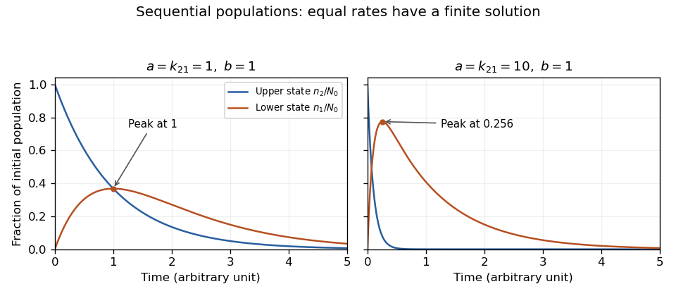
Exact sequential population solutions for coincident and separated loss rates. The equal-rate limit is finite and its lower-state population peaks after the upper-state population has begun to decay.
Details. A polynomial congruence asks for integer residue classes satisfying an equation such asInteger coefficients ensure that replacing by a congruent integer changes by a multiple of . The problem is therefore an equation in the quotient ring , rather than infinitely many unrelated integer tests.
For , the solutions are modulo eight. This quadratic has four roots because the quotient ring has zero divisors: does not force either factor to vanish individually. Over a prime modulus, a nonzero degree- polynomial has at most roots because the quotient is a field. The nonzero-polynomial qualification matters if all coefficients vanish modulo the prime.
For coprime moduli, the Chinese remainder theorem combines solutions componentwise. Thus solving modulo prime powers and then recombining is a natural strategy; lifting between powers of one prime introduces additional conditions, as in Hensel's lemma.
The mitochondrial intermembrane space is the compartment between the outer and inner mitochondrial lipid bilayers, including the spaces within cristae. It is separated from the mitochondrial matrix by the inner lipid bilayer. During oxidative phosphorylation, respiratory proton pumps transfer hydrogen ions from the mitochondrial matrix toward this compartment. Return through ATP synthase couples the resulting proton-motive force to ATP synthesis. The relevant stored energy includes both an electrical potential difference and a chemical concentration difference. [ref]
Molecular Biology of the Cell, 4th edition by Bruce Alberts and others. Chapter 14, The Mitochondrion: proton gradient and ATP synthesis
The compartment also contains cytochrome c, an electron carrier associated with the outer face of the inner lipid bilayer. Its release into the cytosol can contribute to apoptosis. In a cell-free study, depletion of cytochrome c reduced apoptotic activity and add-back restored it, connecting loss of compartmentalization to a new biochemical function. [ref]
Induction of apoptotic program in cell-free extracts: requirement for dATP and cytochrome c by X. Liu and others. 1996, abstract: cytochrome c depletion, add-back and release
Microtomy prepares thin physical sections with a microtome, exposing interior structure for microscopy. The knife separates a layer from a supported specimen while a controlled feed determines the nominal depth increment. Physical section thickness, section orientation and cutting-induced deformation all enter the interpretation of an image. Ultramicrotomy is the specialized thin-section technique used in applications such as transmission electron microscopy.
The preparation method also serves materials research. Yale's instrument description lists a Leica Ultra UC7 with a trimming mill and glass knife maker, and identifies polymers, material fibres and soft metals among suitable specimen materials.[ref]
Microtome at the Yale Institute for Nanoscience and Quantum Engineering. About the instrument, accessories and material list
Manufacturer guidance discusses polymer blends and composite materials, along with the possibility of section compression and cutting artifacts.[ref]Ultramicrotomy Techniques for Materials Sectioning by Leica Microsystems. Opening materials discussion; How to prepare high-quality sections of polymers
A useful teaching experiment would compare cuts through a straight, known circular material fibre at different section orientations. A normal vector to the cut aligned with the fibre axis gives a circular profile. An oblique cut gives an ellipse even when the fibre has suffered no deformation. Image the recovered sections with an optical microscope, measure profile dimensions with an established image stack axis calibration, and record the angle between the section's normal vector and the fibre axis. This tests the geometry of the section rather than assuming that every measured elongation is a physical distortion.
For an original ideal calculation, model the fibre boundary as an infinite circular cylinder of radius , with axis along the unit vector , where . Parallel section planes have equation . The squared Euclidean distance to the axis is , obtained by subtracting the squared axial orthogonal projection from . At the section plane, the boundary therefore satisfiesThis oblique section of a circular cylinder is an ellipse with semi-major and semi-minor axes and areaThe area of an ellipse gives the last expression. For chosen and , the semi-major and semi-minor axes are approximately and . The profile area is times the perpendicular-profile area, an increase of about 41.4 percent entirely explained by section orientation.
The center of an ellipse in this model has coordinate . In an ordered image stack, two sampled section planes separated by consequently have lateral centre displacement . At the chosen and , this displacement is . Here is the spacing between sampled planes, which can differ from the physical section thickness if some sections are not imaged.
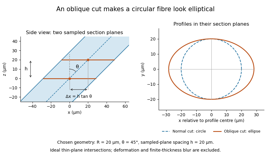
The calculation assumes a circular, straight fibre, known section geometry and negligible physical section thickness relative to resolved features. One elliptical profile alone cannot distinguish an oblique circular fibre from a differently shaped fibre or an unknown deformation. Comparing known reference features and following their positions through an image stack provides additional evidence. Image registration can align images, but an inferred shift may contain real specimen geometry as well as instrument motion; removing every shift would erase the tilt information in this example.
Laser capture microdissection selects small regions or cell populations from a tissue section under microscope guidance, using a laser-mediated collection step. Its purpose is to connect visible histology with molecular measurements from a chosen location. Selection is not the same as preparing the original thin section, and a visible target boundary does not by itself guarantee pure or complete recovery.
The 1996 demonstration by Michael R. Emmert-Buck and colleagues placed a transparent ethylene-vinyl acetate thermoplastic film against a section on a glass slide. A carbon dioxide laser pulse activated the film locally above the desired cells. Focal adhesion enabled transfer of the selected tissue. The reported mechanism was capture by the activated film, rather than simply assuming that the target cells were vaporized. Other laser-assisted cutting arrangements need not use that same transfer mechanism.[ref]
Laser capture microdissection by Michael R. Emmert-Buck and others. Abstract, Science274 (1996), pp.998–1001: film, carbon-dioxide pulse and focal adhesion
The original paper demonstrated amplification of recovered DNA and RNA and recovery of enzyme activity. Those tests connect the collection apparatus with useful downstream assays; they do not prove that every molecular species survives equally or that every captured region consists of one cell type.[ref]
Laser capture microdissection by Michael R. Emmert-Buck and others. Abstract: amplification and enzyme recovery
An original selection model separates purity from yield. Suppose a section contains 100 target cells and 900 background cells. If capture retains of targets but of background, the recovered group has 80 targets and 9 background cells. Target purity is , while target recovery is . Enrichment can therefore be strong even when some desired cells are lost. In general, with initial target fraction and capture probabilities ,provided the denominator is positive. This model assumes independent per-cell accounting, not that an actual laser footprint captures each cell independently.
A measurement record can preserve specimen images before and after collection, the intended boundaries and an assay-specific blank. Images can show spatial removal; a blank can reveal film or collection-background contributions. Target purity versus cell-state change in microdissection then explains why a molecular signal increase after collection may reflect altered population composition rather than altered expression within each target cell.
Preparation time is a separate experimental variable. The RNA-preservation study by Mathieu Clément-Ziza and colleagues tested dry-environment and ethanol-based methods while measuring RNA integrity over the collection period. Keeping a recognizable histological staining pattern and recovering intact RNA are related requirements, but they are distinct measurements.[ref]
Stabilization of RNA during laser capture microdissection by performing experiments under argon atmosphere or using ethanol as a solvent in staining solutions by Mathieu Clément-Ziza and others. Abstract and Figures1–2: RNA-quality comparison and visual selection
Target purity versus cell-state change in microdissection is the distinction between changing which cells enter an assay and changing the molecular state of the target cells themselves. Microdissection can enrich a selected cell population while its per-cell gene expression stays unchanged. Conversely, a measured change can combine enrichment, a genuine cell state difference and altered molecular recovery during preparation.
An original two-population model makes the ambiguity explicit. For equal per-cell weighting, let be the target-cell fraction and the target and background per-cell signals. The measured mean isWith and , changing from to raises from to without any target-cell change. If the target signal instead falls to at the second measurement, is still , above its original . A rising mixture signal therefore does not establish increased expression within the target cell population.
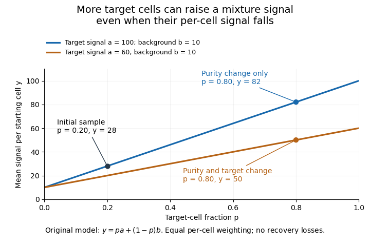
Original two-population model separating enrichment from per-cell signal change during microdissection
. Lines are stipulated mixture equations, not experimental observations. The initial point is p=0.20, a=100, b=10; the two final points share p=0.80 but have different target-cell signals. Details.If and are independently known, then . Holding those inputs fixed, a small signal error propagates as . Purity amplifies that error fivefold, whereas amplifies it by only . Estimating purity is useful, but an uncertain purity or an unrepresentative background introduces further error.
Normalization also changes the mixing weights. If target and background cells contribute total extracted RNA amounts per cell, their fraction of the extracted RNA isAt and , of the RNA comes from target cells despite target-cell purity. A signal per unit total RNA is therefore not automatically the same observable as a signal per starting cell.
Preparation can alter the analyte without creating an original in-vivo cell state difference. In a primary study, Mathieu Clément-Ziza and colleagues compared conditions preserving RNA integrity during laser capture microdissection, including an argon atmosphere and an ethanol-based preparation. Their time-dependent RNA-quality measurements address preservation, not proof that all living-cell transcription stayed unchanged.[ref]
Useful comparisons separately document selected regions, target fraction, recovery and the normalization denominator. Before/after specimen images test what was removed; molecular quality controls test what survived; matched biological comparisons test the proposed cell state change. No one of those observations substitutes for all the others.
Pinned article: Introduction to the OurBigBook Project
Welcome to the OurBigBook Project! Our goal is to create the perfect publishing platform for STEM subjects, and get university-level students to write the best free STEM tutorials ever.
Everyone is welcome to create an account and play with the site: ourbigbook.com/go/register. We belive that students themselves can write amazing tutorials, but teachers are welcome too. You can write about anything you want, it doesn't have to be STEM or even educational. Silly test content is very welcome and you won't be penalized in any way. Just keep it legal!
Intro to OurBigBook
. Source. We have two killer features:
- topics: topics group articles by different users with the same title, e.g. here is the topic for the "Fundamental Theorem of Calculus" ourbigbook.com/go/topic/fundamental-theorem-of-calculusArticles of different users are sorted by upvote within each article page. This feature is a bit like:
- a Wikipedia where each user can have their own version of each article
- a Q&A website like Stack Overflow, where multiple people can give their views on a given topic, and the best ones are sorted by upvote. Except you don't need to wait for someone to ask first, and any topic goes, no matter how narrow or broad
This feature makes it possible for readers to find better explanations of any topic created by other writers. And it allows writers to create an explanation in a place that readers might actually find it.
Figure 1. Screenshot of the "Derivative" topic page. View it live at: ourbigbook.com/go/topic/derivativeVideo 2. OurBigBook Web topics demo. Source. - local editing: you can store all your personal knowledge base content locally in a plaintext markup format that can be edited locally and published either:This way you can be sure that even if OurBigBook.com were to go down one day (which we have no plans to do as it is quite cheap to host!), your content will still be perfectly readable as a static site.
- to OurBigBook.com to get awesome multi-user features like topics and likes
- as HTML files to a static website, which you can host yourself for free on many external providers like GitHub Pages, and remain in full control

Figure 2. You can publish local OurBigBook lightweight markup files to either OurBigBook.com or as a static website.
Figure 3. Visual Studio Code extension installation.
Figure 5. . You can also edit articles on the Web editor without installing anything locally. Video 3. Edit locally and publish demo. Source. This shows editing OurBigBook Markup and publishing it using the Visual Studio Code extension. 
- Infinitely deep tables of contents:




All our software is open source and hosted at: github.com/ourbigbook/ourbigbook
Further documentation can be found at: docs.ourbigbook.com
Feel free to reach our to us for any help or suggestions: docs.ourbigbook.com/#contact