Topics (384k) Articles (398k) Users (410) Discussions (242) Comments (383) Files (13k) New article

Pulse-echo imaging sends a short acoustic pulse and records echoes returning from interfaces or scatterers. If sound speed is approximately constant and the path is straight, an echo delay corresponds to range , because sound travels to the scatterer and back.
Scanning beam direction and measuring echo strength produces an image. Pulse duration and bandwidth affect axial resolution, while beam width affects transverse resolution. Incorrect sound-speed assumptions distort inferred positions, and multiple reflections can create echoes that do not correspond to a single direct round trip.
Positive-pressure ventilation assists inhalation by raising pressure at the airway opening, driving gas into the lungs when that pressure exceeds alveolar pressure. It differs mechanically from spontaneous expansion of the thorax or negative-pressure ventilation, which lowers pressure around the lungs to produce the relevant distending difference. A ventilator's mask or tube supplies the applied airway connection.[ref]
The direction of flow still depends on a pressure difference, not on whether either pressure is above atmospheric. For a simple resistive path,with positive directed inward and the airway resistance. In an original example, pressures 10 and 8 cm HO and cm HO·s/L give inward flow 0.5 L/s. Pressures 8 and 10 cm HO give outward flow 0.5 L/s. Both pairs are positive relative to atmosphere.
This explains why positive end-expiratory pressure can coexist with exhalation. The applied pressure can remain above atmospheric while elastic recoil produces a still higher alveolar pressure and drives gas outward. At equal opening and alveolar pressures, the same ideal resistive model gives zero flow.
The resulting tidal volume also depends on respiratory-system compliance, airway resistance, duration and any active respiratory muscle effort. The no-flow interval used to interpret plateau airway pressure removes one resistive contribution only under the required measurement conditions.[ref] Positive pressure is therefore a mode of applying mechanical assistance, not a guarantee of a particular inward flow, volume or gas-exchange result.
A ventilator is a machine that assists or replaces pulmonary ventilation by supplying a controlled gas-delivery path to the lungs. The interface can be a mask or a breathing tube; the machine and interface together support mechanical ventilation.[ref] Gas delivery, oxygen concentration and respiratory mechanics remain distinct parts of that support.
A useful engineering description separates the commanded quantity from the measured response. A machine can regulate an applied pressure or a flow history while monitoring pressure and gas volume. Its displayed or reconstructed quantities depend on sensors, timing and the selected model. The manufacturer's treatment of plateau airway pressure, for example, distinguishes a hold measurement from computed monitoring estimates and states conditions under which they are available.[ref]
Measured values for Ppeak and Pplateau by Hamilton Medical. Principles of measuring plateau pressures; Monitoring parameter Pplateau
An original circuit example shows why upstream delivered volume need not equal the volume entering the patient. In a simplified volume balance,If a stipulated source supplies 0.50 L, ventilator circuit compliance stores 0.04 L during pressurization, and 0.06 L escapes through a leak, only 0.40 L reaches the modeled patient compartment. This is an illustrative uncompensated circuit, not a description of every ventilator's displayed tidal volume.
The stored term can be approximated as . A stipulated compliance of 2 mL/cm HO with a 20 cm HO pressure rise gives the stated 40 mL. Measuring volume at another location, or compensating for known circuit properties, changes what is being reported.
A ventilator consequently supplies an experimentally testable physical system: gas path, actuation, sensors and control logic. A pressure or volume setting alone is not a complete observation of alveolar gas renewal, especially when flow, leakage or circuit storage changes.
Negative-pressure ventilation assists inhalation by reducing the pressure outside the chest relative to that at the airway opening. A chamber encloses the torso while the mouth and nose communicate with gas outside the chamber. Lower external pressure allows chest expansion and makes alveolar pressure transiently lower than the airway opening, drawing gas into the lungs.
The original 1929 apparatus report by Philip Drinker and Louis A. Shaw describes a sheet-metal tank, a sealing neck collar and the head supported outside the tank. Alternating tank pressure moved the chest while the head remained exposed to atmospheric pressure.[ref]
An apparatus for the prolonged administration of artificial respiration: I. A design for adults and children by Philip Drinker and Louis A. Shaw. Pages 230–231, Figures 1–2
This is a concrete distinction between applying a pressure change to the body surface and applying it through an airway interface.An original static example uses transpulmonary pressure . With an open airway and no flow, suppose alveolar pressure is zero on an atmospheric gauge. Changing pleural pressure from to cm HO raises from 6 to 10 cm HO. For stipulated lung compliance L/cm HO, the linear model predictsDuring the actual filling transient, pressure differences also overcome airway resistance. The static calculation does not predict the instantaneous flow waveform.
Tank pressure is a boundary condition, not a direct measurement of pleural pressure. Chest-wall mechanics and body geometry affect pressure transmission. Consequently, an equal numerical pressure at a positive-pressure airway interface and a negative-pressure body chamber need not produce identical volume changes or circulatory effects. The useful unifying quantity for lung distension is the pressure difference across the lung, together with its mechanical response.
A mechanical impedance measurement determines the amplitude and phase of driving force relative to motion at a specified port. With the convention , a driving-point test measures the force and velocity at the same location and in the same direction. Both terminal motions must be included if the second terminal moves. Ole Døssing's manufacturer guide describes this need for coincident excitation/response measurements and the use of an impedance head combining force and acceleration sensing.[ref]
Structural Testing Part I: Mechanical Mobility Measurements by Ole Døssing. “Response Measurements”, printed pp.30–32, driving-point transducer arrangement
A typical apparatus uses a vibration exciter or instrumented impact to drive the structure, a force transducer in the excitation path, an accelerometer near the driving point, and synchronized acquisition of both signals. The measurement calibration, mounting, excitation range and fixture motion belong in the test description. A transfer response at a remote point is useful but answers a different question from driving-point mechanical impedance.
For a steady sinusoid with convention , acceleration complex amplitude gives , henceFor example, at let the applied force amplitude be and acceleration amplitude be in phase with the force. Then and . This is the response of a pure mass: force leads velocity by a quarter cycle. Reporting only the two amplitudes would lose that distinction from a dissipative response.
For broadband excitation, estimate the relevant frequency response from the synchronized force and response records, with suitable error analysis. A response peak alone can come from a peak in the applied force, so the response spectrum by itself does not establish structural resonance. Transducer mass can modify a small structure, and fixture inertia can contribute measured force; both require an explicit measurement model. Repeating at another excitation amplitude tests the assumed linear regime rather than treating a changed response ratio as the same invariant system property.[ref]
Structural Testing Part I: Mechanical Mobility Measurements by Ole Døssing. “The Frequency Response Function”, p.14; “Errors”, pp.23–25; “Response Measurements”, pp.30–32; “Calibration”, p.43
Mechanical driving-point mobility is the frequency response relating motion to excitation at the same mechanical port. Using relative velocity and signed entering force , its zero-initial-state Laplace transform convention iswhere is the force/velocity mechanical driving-point impedance. Mobility has units . The measured direction, port and boundary conditions are part of its specification.[ref]
Structural Testing Part I: Mechanical Mobility Measurements by Ole Døssing. “Mobility Measurements — Definitions”, printed p.16
For an inertial element , dashpot coefficient and spring stiffness sharing a port,For complex amplitudes, mobility tends to at low frequency when and to at high frequency when . A spring therefore prevents a nonzero steady drift response to constant force. This differs from the steady mechanical mobility of a body under pure linear drag, which has no elastic restoring term.
Take , and . At the reactive terms cancel and . A peak force amplitude gives peak velocity and mean entering power . These statements concern the same port; a response measured elsewhere is a transfer mobility.
A response/force ratio using acceleration instead is mechanical accelerance, ; using displacement gives mechanical receptance, . Confusing these ratios introduces a frequency-dependent magnitude and phase error. With several coupled ports, matrix inversion rather than elementwise reciprocation is needed to exchange complete impedance and mobility descriptions.
Transducer sensitivity describes how much the output of a measuring transducer changes when its input changes. For an output responding smoothly to input , a local model usesVIM defines sensitivity of a measuring system through the quotient of corresponding indication and input changes, noting that sensitivity can depend on the input value and that the changes used must be appreciable relative to resolution.[ref] The derivative is the smooth local limit of that response ratio.
For an original pressure-to-potential transducer, stipulateIts transducer sensitivity isAt , the output is and the sensitivity is . Across the finite interval from to , output changes by , so the measured response ratio is instead . Specify the operating point or interval rather than treating these two slopes as contradictory.
An output increment corresponds locally to input-referred resolution at the first operating point. This conversion is not a complete uncertainty statement. Increasing electronic gain can enlarge output noise as well as the signal; detector saturation can flatten the response and destroy local invertibility.
Estimate transducer sensitivity with known input steps, repeated outputs and checks for changing zero, loading and temperature. In a linear response , a constant offset cancels from differences; a changing offset does not. Retain both the sensitivity relation and its uncertainty in measurement calibration, and propagate the relevant contributions when reporting a measurement result.
A Bourdon tube is a curved, hollow elastic element that converts a pressure difference into movement of its free end. A common form has an oval tube cross-section and a roughly C-shaped centreline. Fluid pressure is applied through the fixed end, while the other end is closed and free to move. WIKA describes the cross-section tending toward a more circular shape under internal pressure and the resulting end motion being transmitted to a pointer.[ref]
Elastic element pressure gauges by WIKA. IN00.01,09/2010, p1, Pressure gauges with bourdon tube and labelled mechanism
In a Bourdon tube pressure gauge, the tube, linkage, gearing and pointer form a mechanical measuring chain. The sensing element undergoes elastic deformation; the movement converts a small displacement into a readable measurement indication. A steady pressure reading does not require continuous flow through the closed tube.
For an original small-range model, let free-end displacement be , with gauge pressure and stipulated . Let the linkage produce pointer angle with . At ,The combined response is . These are illustrative coefficients, not a specification for a WIKA instrument. The actual response depends on tube geometry, material and movement.
The reference pressure belongs in the interpretation. With the outside of the element exposed to local atmosphere, the response measures gauge pressure, rather than absolute pressure. WIKA separately describes sealed reference arrangements for absolute-pressure instruments.[ref]
Elastic element pressure gauges by WIKA. p1, Description, atmospheric reference; p3, Absolute pressure gauges
For instrument calibration, connect the gauge and a suitable measurement standard to a common pressure source, allow equilibration, and compare several increasing and decreasing pressures within the intended range. Record the relative height of fluid-filled pressure ports because hydrostatic pressure can add a difference between them. Differences between increasing and decreasing readings can reveal hysteresis or backlash; a zero shift after loading can reveal a changed mechanical state. The original linear model alone does not establish the gauge's measurement uncertainty.
Detector responsivity relates a detector's output to the incident radiant input under stated conditions. For a photodiode illuminated at a specified wavelength, current spectral responsivity iswhere is the background current and is incident optical power. Its units are . NIST's detector-calibration publication develops spectral radiant-power responsivity as the quantity transferred from optical standards to photodetectors.[ref]
For an original example, incident power produces net photocurrent, giving . If readout electronics convert that current to , the complete system's voltage responsivity is . A value without its output quantity and units can therefore be misleading.
For a photodiode with no internal multiplication, let quantum efficiency be collected electrons per incident photon. A photon has energy , with Planck constant , speed of light and elementary charge . Thus a photon arrival rate gives and net current . ThereforeAt , the original example corresponds to . This relation assumes the stated charge-collection model; internal gain changes the interpretation.
Responsivity can depend on wavelength, irradiation geometry, bias and temperature. Detector linearity tests whether a response ratio stays constant as input level changes; detector saturation can make it strongly level-dependent. In a nonlinear response, the ratio of corrected output to input and the local transducer sensitivity are different quantities. Retain the wavelength, beam conditions, readout convention and measurement uncertainty when reporting a responsivity measurement.
A thermoelectric offset is an unwanted electric potential difference associated with Seebeck effect responses in a measurement circuit. Dissimilar conductors at different junction temperatures can generate a signal even when the intended electrical input is absent. Keithley's handbook discusses these offsets as a major limitation in low-voltage and low-resistance measurements.[ref]
Low Level Measurements Handbook, Seventh Edition by Keithley Instruments. §3.2.2, thermoelectric EMFs; §3.3.2, offset compensation
For a simple two-material circuit, a useful model iswhere the Seebeck coefficients depend on conductor material and temperature. With a stipulated constant difference and junction-temperature difference , the offset is . These are teaching inputs, not coefficients assigned to a particular real connector pair.
That small offset can dominate an intended signal. For an original resistor tested at , the wanted drop is also . An additive offset of the same sign doubles the indication to and gives an apparent if it is ignored. Reversing the current produces readings and in this model; their half-difference recovers the wanted .
Polarity reversal measurement cancels the unchanged offset, not every temperature effect. Thermal changes during the cycle can leave a residual, while current-induced heating can alter the resistor itself. The handbook therefore connects reversal timing with thermal stability.[ref]
Low Level Measurements Handbook, Seventh Edition by Keithley Instruments. §3.3.2, current-reversal method and thermal-time-constant condition
An offset investigation records connector materials, junction temperatures, warm-up and handling, and compares readings before and after reversal. Reducing temperature gradients and avoiding unnecessary dissimilar-metal connections can reduce the generated signal. Keep residual correction uncertainty in the measurement result. A thermoelectric offset and random thermal noise have different roles in the measurement model; they are not interchangeable merely because both involve temperature.
A reproducibility condition of measurement belongs to a declared set of conditions used to assess measurement reproducibility. The VIM set includes different locations, operators and measuring systems, with replicate measurements on the same or similar objects. The systems may also use different measurement procedures; the specification should identify both changed and unchanged conditions.[ref]
For an original physical comparison, laboratories A and B measure the same stable reference block's length at a stated reference temperature. Each laboratory uses its own operator and differential length comparator. Record the block identity, temperature observations, applied corrections, procedure version and instrument reference in each result. Measurements before and after transport help distinguish reference changes from laboratory differences.
Suppose the stipulated readings, in millimetres, areThe laboratory means are and , differing by . Each pair has sample standard deviation . Small within-laboratory scatter therefore does not remove the difference between laboratory means.
Because location, operator and system changed together, this comparison alone cannot identify which caused the difference. In a chosen additive measurement model,a difference could be assigned entirely to a system contribution or entirely to a location contribution, with the same predicted means. Separating those explanations needs additional comparisons that vary their combinations.
The conditions describe the experiment's scope; they are not a numerical precision result by themselves. Report the complete measurand and what remained common, including any shared measurement standard. A common reference error can affect both laboratories, so agreement under changed conditions does not by itself establish measurement trueness.
Positioning repeatability describes the scatter of positions reached when a motion system repeatedly returns to the same commanded position under specified conditions. It is an application of measurement repeatability, a form of measurement precision. A system may return to almost the same wrong position each time, so small scatter does not establish measurement accuracy.[ref]
International vocabulary of metrology by JCGM. VIM3 entries2.15,2.20 and2.21: precision and repeatability conditions
The approach direction belongs in the test description. Unidirectional positioning repeatability keeps it fixed; bidirectional positioning repeatability includes returns from both directions. To measure the assembled stage, independently observe its final position rather than only the motor's rotary encoder count. Physik Instrumente describes a static test that lets the platform stop before reading it, using an interferometer for displacement and an autocollimator for angular error, with two reflecting mirrors on the stage.[ref]
How to Consistently Verify the Performance of Nanopositioning Motion Control Equipment by Physik Instrumente. §§3.1–3.2, static readout, direction convention and paired-mirror apparatus
For an original numerical example, repeatedly command . Suppose an independent position readout with known measurement calibration gives the errors , in micrometres,Each direction has the same sample standard deviation,Yet their arithmetic means are 0 and . The magnitude of their mean difference, a positioning reversal error at this target, is 2.0 micrometres, far larger than the within-direction scatter. Pooling all eight values gives a sample standard deviation of ; that statistic mixes the directional shift with the smaller return-to-return variation.
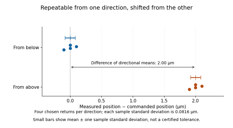
Two tightly repeated return positions separated by approach direction
. Original chosen errors at one target. Four trials per direction; small bars show mean plus or minus one sample standard deviation. The figure is not measured product performance. Details.The calculation uses a declared sample standard deviation, not an unspecified manufacturer's tolerance or a universal repeatability convention. A positioning specification must state its approach directions, target positions, settling/readout procedure, load, environmental conditions, statistic and measurement uncertainty. A single target does not establish performance over the travel range. The manufacturer's method explicitly separates directional means from scatter and combines information from multiple targets when forming axis-level specifications.[ref]
Backlash is one possible cause of direction-dependent behavior, while thermal expansion and instrumental drift can move the apparent target over time. A repeatability experiment must distinguish those effects from random scatter. Measuring small returns to one target also answers a different question from minimum incremental motion, which asks whether a small commanded change can actually be executed.
A repeatability condition of measurement belongs to a specified set of conditions used to assess measurement repeatability. The VIM set includes a common measurement procedure, operator, measuring system, operating conditions and location, with repeated measurements of the same or similar objects over a short period.[ref] A condition is therefore meaningful relative to the whole declared set, rather than being a property supplied by the word repeat alone.
For a physical length experiment, specify one operator, one differential length comparator, a reference block, the contact orientation, the remove-and-replace cycle, the settling rule and a short session after thermal equilibration. Keep the measurement calibration fixed during that series. Record every completed measurement, including the elapsed time and block temperature. Reading the unchanged display repeatedly and replacing the block between readings are different measurement procedures, even if the displayed numbers happen to coincide.
An original thermal calculation explains why the operating conditions matter. Suppose a metal reference block has length at , with stipulated constant linear thermal expansion coefficient . In the small-expansion model,A temperature rise of changes its length by . If the intended measurand is length at , that change requires an appropriate correction; it should not be silently interpreted as random comparator scatter. This calculation holds other thermal effects fixed and does not model expansion of the comparator itself.
The same room and a short elapsed time do not prove that the relevant conditions were stable. Record observed deviations and assess their effect. Deliberately varying operators over several days at the same location leads to a study of intermediate measurement precision; varying locations and measuring systems leads toward measurement reproducibility.
A primary reference measurement procedure determines a result without calibration against a measurement standard for a quantity of the same kind. It can still depend on calibrated measurements of other quantities. The VIM example determines delivered liquid volume from a mass difference and liquid mass density, rather than comparing it with another calibrated delivered volume.[ref]
For an original ideal calculation, let the receiving vessel's tare mass be and its gross mass after delivery be . Suppose the liquid's mass density at the measurement conditions is . ThenWith independent standard uncertainties and ,so . These are stipulated values, not a recommended liquid or an actual calibration result.[ref]
The physical procedure would weigh the receiver before and after delivery, establish the liquid temperature and density, and include significant corrections in its measurement model. Evaporation, buoyancy and correlated mass readings can invalidate the simplified expression above. Primary describes the reference relation, not freedom from measurement uncertainty or the absence of any instrument calibration. Its primary status is therefore a claim about the complete procedure, not about this equation alone.
Pinned article: Introduction to the OurBigBook Project
Welcome to the OurBigBook Project! Our goal is to create the perfect publishing platform for STEM subjects, and get university-level students to write the best free STEM tutorials ever.
Everyone is welcome to create an account and play with the site: ourbigbook.com/go/register. We belive that students themselves can write amazing tutorials, but teachers are welcome too. You can write about anything you want, it doesn't have to be STEM or even educational. Silly test content is very welcome and you won't be penalized in any way. Just keep it legal!
Intro to OurBigBook
. Source. We have two killer features:
- topics: topics group articles by different users with the same title, e.g. here is the topic for the "Fundamental Theorem of Calculus" ourbigbook.com/go/topic/fundamental-theorem-of-calculusArticles of different users are sorted by upvote within each article page. This feature is a bit like:
- a Wikipedia where each user can have their own version of each article
- a Q&A website like Stack Overflow, where multiple people can give their views on a given topic, and the best ones are sorted by upvote. Except you don't need to wait for someone to ask first, and any topic goes, no matter how narrow or broad
This feature makes it possible for readers to find better explanations of any topic created by other writers. And it allows writers to create an explanation in a place that readers might actually find it.
Figure 1. Screenshot of the "Derivative" topic page. View it live at: ourbigbook.com/go/topic/derivativeVideo 2. OurBigBook Web topics demo. Source. - local editing: you can store all your personal knowledge base content locally in a plaintext markup format that can be edited locally and published either:This way you can be sure that even if OurBigBook.com were to go down one day (which we have no plans to do as it is quite cheap to host!), your content will still be perfectly readable as a static site.
- to OurBigBook.com to get awesome multi-user features like topics and likes
- as HTML files to a static website, which you can host yourself for free on many external providers like GitHub Pages, and remain in full control

Figure 2. You can publish local OurBigBook lightweight markup files to either OurBigBook.com or as a static website.
Figure 3. Visual Studio Code extension installation.
Figure 5. . You can also edit articles on the Web editor without installing anything locally. Video 3. Edit locally and publish demo. Source. This shows editing OurBigBook Markup and publishing it using the Visual Studio Code extension. 
- Infinitely deep tables of contents:



All our software is open source and hosted at: github.com/ourbigbook/ourbigbook
Further documentation can be found at: docs.ourbigbook.com
Feel free to reach our to us for any help or suggestions: docs.ourbigbook.com/#contact