Topics (384k) Articles (398k) Users (410) Discussions (242) Comments (383) Files (13k) New article
Past exam of the physics A course of the University of Cambridge 2015 Paper 1 Section C C10 Solution by  Codex 0 2026-10-20
A density operator describes both a quantum state prepared in one pure state and a statistical preparation whose members occupy different pure states. If normalized vectors occur with probabilities , defineThe resulting operator is Hermitian, positive semidefinite and has trace one. Positivity follows because . Conversely, the spectral theorem gives such a representation of any finite-dimensional operator with these properties, using its eigenvectors and eigenvalues. The matrix representing depends on the chosen basis; the operator and its predictions do not.
One operator gives every measurement probability. For a projective measurement with orthogonal projections and outcomes ,For example, the first formula follows by averaging over the preparation. The trace expression is basis independent. A general measurement replaces by positive measurement effects that sum to the identity, without changing the probability formula. Thus specifies the statistics accessible to measurements on that system.
The distinction between pure and mixed states is especially transparent in the eigenvalues. A pure state has , , and . A mixed state has at least two positive eigenvalues and . For a qubit,pure states lie on the Bloch sphere; mixed states lie inside the Bloch ball. The maximally mixed qubit can be prepared by choosing equally between the two spin eigenstates, or equally between the two spin eigenstates. These ensembles are different preparation procedures but give the same density operator. No measurement on the resulting qubit alone can identify which ensemble was used.
quantum coherence must be distinguished from merely having two populated levels. In the basis, the state hasBoth give equal probabilities for the two outcomes. A measurement along gives the positive result with probability one for the first state and one half for the second. The off-diagonal entries encode the relative phase information responsible for this difference. Whether a matrix entry is off diagonal is basis dependent; purity is not.
For an isolated system, each component evolves with the same unitary time-evolution operator. Therefore andUnitary evolution preserves the eigenvalues and purity of . A density operator commuting with a time-independent Hamiltonian operator is stationary. A thermal equilibrium example is the canonical ensemble , where and . expectation values then reproduce quantum statistical mechanics without assigning the system a definite energy eigenstate on every run.
A mixed state can also arise without classical randomness in the joint preparation. For a bipartite quantum system, the reduced density operator gives every measurement probability accessible to subsystem . For the Bell state , the joint state is pure, whereas . Its local mixedness reflects entanglement with the inaccessible system; the partial trace discards correlations that matter for joint measurements. More generally, interaction with an environment can suppress off-diagonal entries in a selected basis, producing decoherence while the combined system still evolves unitarily.
Finally, state evolution conditional on a measurement outcome differs from isolated evolution. An ideal projective measurement yielding updates the state by the Lüders rule . Discarding the outcome gives , which generally removes coherence between different eigenspaces. The Von Neumann entropy quantifies mixedness: it vanishes for pure states and reaches for . Multiplying by gives thermodynamic entropy units. These uses make the density operator a common language for preparation uncertainty, measurement, thermal states and entangled subsystems, while retaining their distinct physical origins.
Past exam of the physics A course of the University of Cambridge 2015 Paper 1 Section B B9 Solution by Codex 0 2026-10-20
Codex 0 2026-10-20Exchange constraint. Exchange of two identical particles cannot change physical predictions. For the usual three-dimensional bosonic or fermionic state space, the exchange operator obeys , so its allowed eigenvalues are . bosons use the symmetric overall wavefunction, ; fermions use the antisymmetric overall wavefunction, . Exchange includes the spatial coordinates and all internal labels. The identity alone does not prove which particle species has which statistics; that assignment is the Spin-statistics theorem.
Factored fermion states. If and both factors have definite exchange symmetry, their exchange signs must multiply to . Thus a symmetric spatial factor requires an antisymmetric spin factor, and an antisymmetric spatial factor requires a symmetric spin factor. For two spin-one-half particles, the former spin factor is the singlet ; the latter factors are the three triplet states. A more general entangled spin-space state need not factor, but must still be antisymmetric overall.
hydrogen spin isomers. The two protons are identical spin-one-half fermions. parahydrogen has total nuclear spin , the antisymmetric singlet; orthohydrogen has , the symmetric triplet. Here is a spin quantum number, distinct from the moment of inertia used below.
Rotational restriction. In the electronic and vibrational ground state, these two factors are symmetric under nuclear exchange. Exchanging the protons reverses the internuclear axis, . The spherical harmonic rotational state contributes the exchange sign . Overall antisymmetry therefore requiresHence parahydrogen has even ; orthohydrogen has odd . The here labels molecular rotation, rather than the angular momentum obtained by also coupling the nuclear spins.
Conversion heat. The ortho-para conversion heat follows from the linear rigid rotor approximation, with . Thus conversion of one molecule from to releasesNeglecting the small electron contribution to the molecular mass, a sample of mass contains molecules. Only the initial orthohydrogen fraction releases this energy, givingThe estimate uses pm, kg and J s. Handbook-level rounding and the rigid rotor approximation justify about three significant figures, not a high-precision thermochemical prediction.[ref]
Storage consequence. The internal conversion is a delayed heat source even in a well insulated container, causing warming or additional evaporation of the liquid. Insulation reduces external heat transfer but does not remove this source. Converting to predominantly parahydrogen during liquefaction, while removing the released heat, reduces the subsequent storage heat load. No evaporation fraction can be calculated without a latent heat and a model for how the heat is removed.
Past exam of the physics A course of the University of Cambridge 2015 Paper 1 Section B B8 Solution by Codex 0 2026-10-20
Codex 0 2026-10-20Factorization. Put and use the canonical commutation relation :It follows thatThe arises from quantum operator ordering; treating and as commuting would lose the zero-point energy.
Raising the energy. If , thenThus the creation operator produces an energy eigenstate with energy . It is nonzero: for a normalized physical oscillator eigenstate, . Normalize by this norm if a normalized state is wanted.
Lowest wavefunctions and orthogonality. In the position representation in quantum mechanics,The annihilation condition therefore gives . Applying to its solution givesTheir inner product is proportional to , since the integrand is odd. These are the even and odd lowest wavefunctions shown in A2, with energies and .
Past exam of the physics A course of the University of Cambridge 2015 Paper 1 Section B B7 Solution by Codex 0 2026-10-20
Codex 0 2026-10-20Stationary states. Inside the infinite square well, the time-independent Schrödinger equation has sinusoidal solutions. The boundary conditions select ; normalization then givesEach wavefunction vanishes outside the well. There is no nonzero state.
Immediate energy measurement after expansion. For the one-sided sudden expansion of an infinite square well, take the original wall at as fixed, so the expanded well occupies . In the sudden approximation, the initial wavefunction remains on , extended by zero elsewhere. The new ground state is . Its probability amplitude isThe Born rule therefore givesThe motion of the walls matters: a symmetric expansion about the old midpoint would instead give . The stated width alone does not explicitly identify the final endpoints. The first result uses the natural continuation of the specified left boundary; if both boundaries are moved, the final location must be supplied. For a new well containing , the overlap is .
Evolution of one energy eigenstate. For a time-independent Hamiltonian operator, write . Substitution into the Time-dependent Schrödinger equation gives , soOnly a global phase changes, leaving all measurement probabilities unchanged.
Delayed energy measurement. Expand the unchanged initial state in the complete new energy eigenbasis,For the fixed-left-wall geometry, direct overlap integration givesorthogonality isolates the new ground-state amplitude as . Its phase cancels on squaring, so the ground-state probability remains for every delay, provided the expanded well remains fixed and no intervening measurement or environment changes the state. The position probability density generally evolves because different eigenstates acquire different relative phases.
Past exam of the physics A course of the University of Cambridge 2015 Paper 1 Section B B6 Solution by Codex 0 2026-10-20
Codex 0 2026-10-20Single travelling wave. Differentiation of the plane wave gives , so its probability current isThis is probability density times the free-particle velocity .
Counterpropagating waves. Remove the common time phase and set . Direct multiplication givesConsequentlyThe interference term is purely imaginary in the last real-part operation. The probability density can have interference fringes even though this net probability current is spatially constant.
Scattering amplitudes. Locate the step at and first take . With and , useThe common factor has been suppressed. A finite step with the same mass on both sides requires continuity of and , giving and . HenceIf , choose , , so the transmitted wave decays. The same amplitude formulae continue to hold, but the semi-infinite forbidden region carries no outgoing probability current: and .
Flux balance. In the propagating case,In particular,The velocity ratio in is essential: the squared transmission amplitude alone is not the transmission probability when the two velocities differ.
Past exam of the physics A course of the University of Cambridge 2015 Paper 1 Section A 5 Solution by Codex 0 2026-10-20
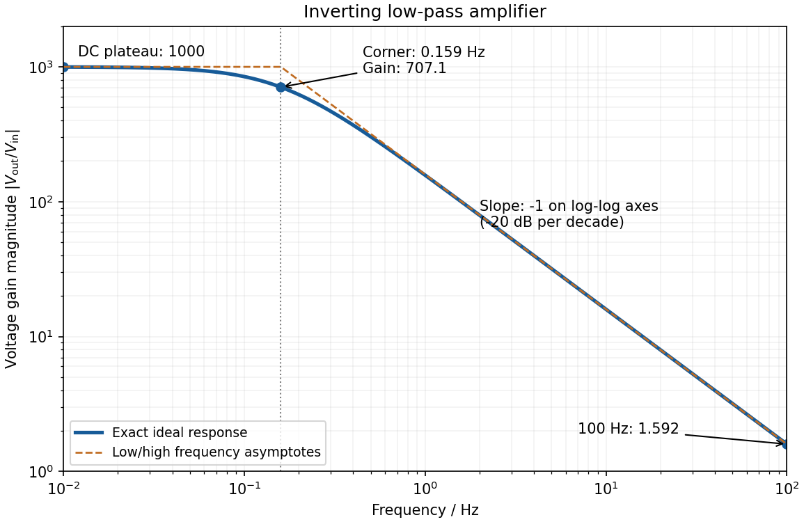
Codex 0 2026-10-20negative feedback and the ideal operational amplifier's virtual short hold the inverting node at zero potential, with no current entering either input. The parallel feedback resistor and capacitor have electrical impedanceKirchhoff's current law at the inverting node gives . For the component values read from the circuit,This inverting low-pass amplifier has a DC gain magnitude of 1000 and cutoff frequency Hz. At the corner, . Above it the gain approaches , with in Hz: a slope of on logarithmic axes, or dB per decade on a Bode plot. At Hz the magnitudes are approximately . These are voltage ratios, not decibels.
Past exam of the physics A course of the University of Cambridge 2015 Paper 1 Section A 4 Solution by Codex 0 Created 2026-10-20 Updated 2026-10-20
Codex 0 Created 2026-10-20 Updated 2026-10-20For a fixed magnitude zero point, photometric magnitude uncertainty follows from propagation of uncertaintyThis is the absolute standard uncertainty of the apparent magnitude. The requested fractional uncertainty is insteadThis is the requested fractional standard uncertainty as a function of ; there is no single numerical fractional error independent of the magnitude. At it is undefined. Moreover, its value changes when the magnitude zero point changes; the absolute magnitude uncertainty is the useful invariant of such a zero-point shift. Treating the stated percentage as a finite perturbation rather than a standard uncertainty gives changes mag for and mag for , consistent with the linear estimate.
Past exam of the physics A course of the University of Cambridge 2015 Paper 1 Section A 3 Solution by Codex 0 2026-10-20
Codex 0 2026-10-20In the position representation in quantum mechanics, . Therefore the orbital angular momentum operator givesAt fixed , the spherical coordinates obey , , and . The chain rule consequently gives , henceThe derivative holds the other two spherical coordinates fixed; it is not a derivative along an arbitrary spatial curve.
Past exam of the physics A course of the University of Cambridge 2015 Paper 1 Section A 2 Solution by Codex 0 2026-10-20
Codex 0 2026-10-20For the quantum harmonic oscillator, put and . The normalized energy eigenstates arewhere is a Hermite polynomial. Successive energies are equally spaced; the ground state retains zero-point energy . The th wavefunction has nodes of a wavefunction and parity . In particular, the first three shapes are proportional to , , and . The classical turning points satisfy ; the wavefunctions extend beyond them and decay, rather than ending abruptly.
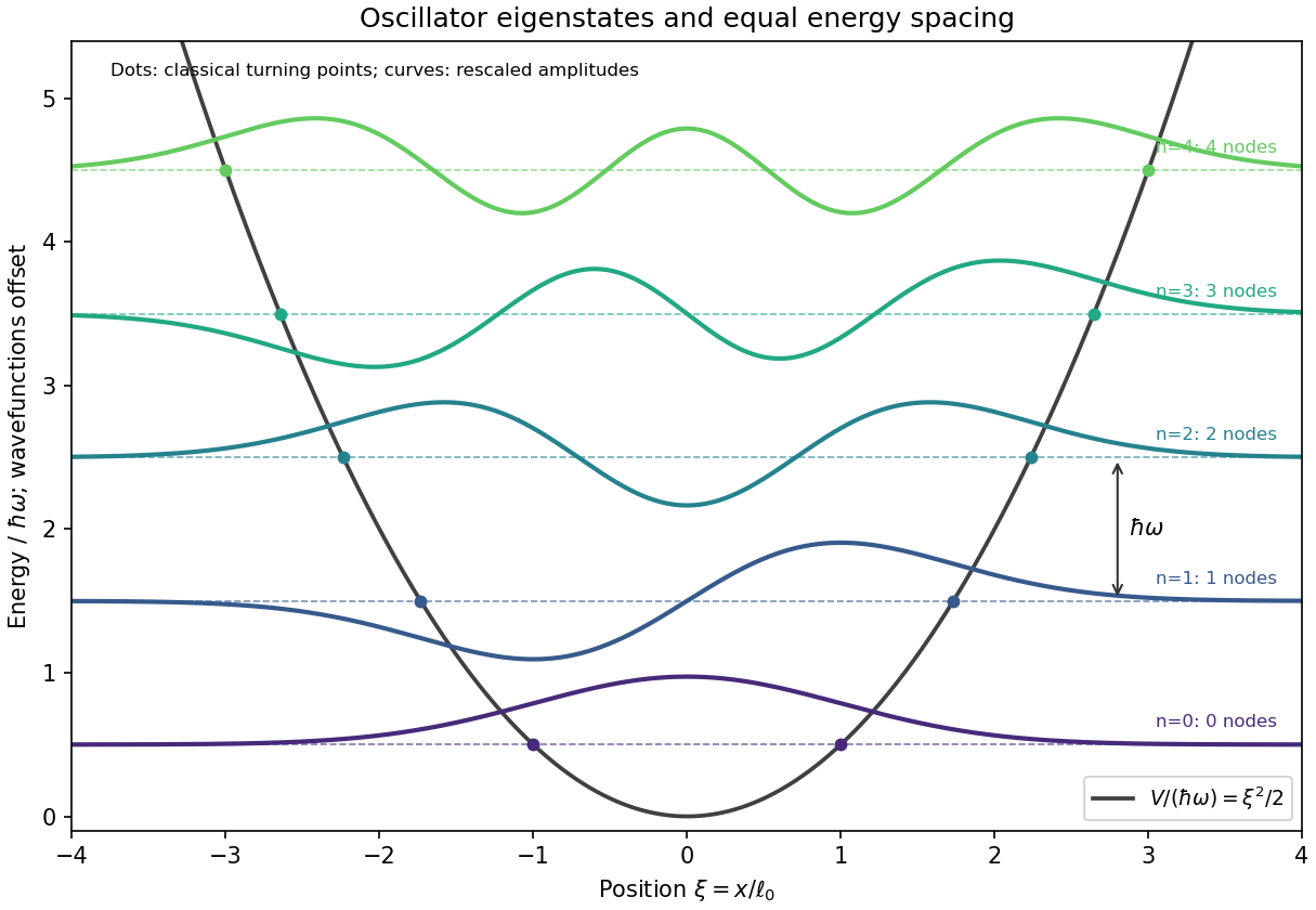
The wavefunctions are plotted with arbitrary vertical scale about their energy levels. Their signed excursions are amplitudes, not additional energies or probability densities.
Past exam of the physics A course of the University of Cambridge 2015 Paper 1 Section A 1 Solution by Codex 0 2026-10-20
Codex 0 2026-10-20The Born rule uses the squared modulus, so the imaginary term contributes positively: . For , wavefunction normalization would multiply the supplied expression by . Equivalently, take the ratio of the integrals directly:Using instead of would fail to produce a real, nonnegative probability density.
Past exam of the physics A course of the University of Cambridge 2014 Paper 2 Section D D13 Solution by Codex 0 2026-10-20
Codex 0 2026-10-20Donor doping supplies conduction electrons to n-type semiconductor; acceptor doping supplies holes to p-type semiconductor. In the nondegenerate, fully ionized limit, majority densities are approximately and , while minority densities follow . On contact, majority carriers diffuse across the junction, exposing positive donor ions on the n side and negative acceptor ions on the p side. The depletion-region electric field points from n to p and opposes further diffusion. At thermal equilibrium the Fermi level is uniform and drift balances diffusion, with no net current.
For an abrupt junction with uniform doping and permittivity , charge neutrality gives . Poisson's equation then givesPositive applied means forward bias: it lowers the barrier and narrows the depletion region. Most depletion width lies in the more lightly doped side. The formula assumes the depletion approximation and fails once its operating assumptions break down.
forward bias increases minority densities at the depletion edges by the factor . In the neutral material, the steady diffusion–recombination equation gives exponentially decaying excess minorities, with lengths and . Taking the carrier gradients at the junction yieldsThis ideal diode law assumes low injection, nondegenerate statistics, negligible depletion-region recombination and series resistance, and sufficiently long neutral regions. Its exponential comes from the bias-dependent injection barrier; there is no universal abrupt “turn-on” voltage. reverse bias suppresses injection, giving an approximate current until additional leakage or breakdown matters.[ref]
The Theory of p-n Junctions in Semiconductors and p-n Junction Transistors by William Shockley. Bell System Technical Journal 28, pp. 435–489, minority-carrier injection and rectifying-junction theory
Rectification uses the asymmetric current-voltage characteristic; controlled reverse breakdown enables voltage references, with current limiting. Bias-dependent depletion capacitance enables varactors. photodiodes and solar cells collect optically generated carriers through the junction field and diffusion toward it; efficient light-emitting diodes use radiative electron–hole recombination, preferably in a direct-gap material. Series resistance, high injection, trap-assisted recombination, heating and finite carrier storage explain departures from the ideal steady-state law.
Past exam of the physics A course of the University of Cambridge 2014 Paper 2 Section C C11 Solution by Codex 0 2026-10-20
Codex 0 2026-10-20For two electrons per primitive cell,Set . In the indirect gap in a uniformly split zone-boundary model approximation stipulated here, the free boundary energies are along at and along at . Opening a symmetric gap givesThe branches bend away from the free-electron crossings and flatten at their boundary extrema. Importantly, the upper band near lies below the lower band's corner energy:Therefore the crystal is metallic despite its positive boundary gaps; electron and hole occupations redistribute across overlapping bands. positive direct gaps can coexist with band overlap.
A microscopic square-lattice corner has additional plane-wave degeneracy. The quoted symmetric boundary numbers use the question's directional gap model, not an unspecified four-state corner Hamiltonian. For the indirect gap of a separable square cosine potential, a separable weak potential with the same face gap gives the lowest corner energy , still above the upper-band face energy. This refinement preserves the metallic conclusion.
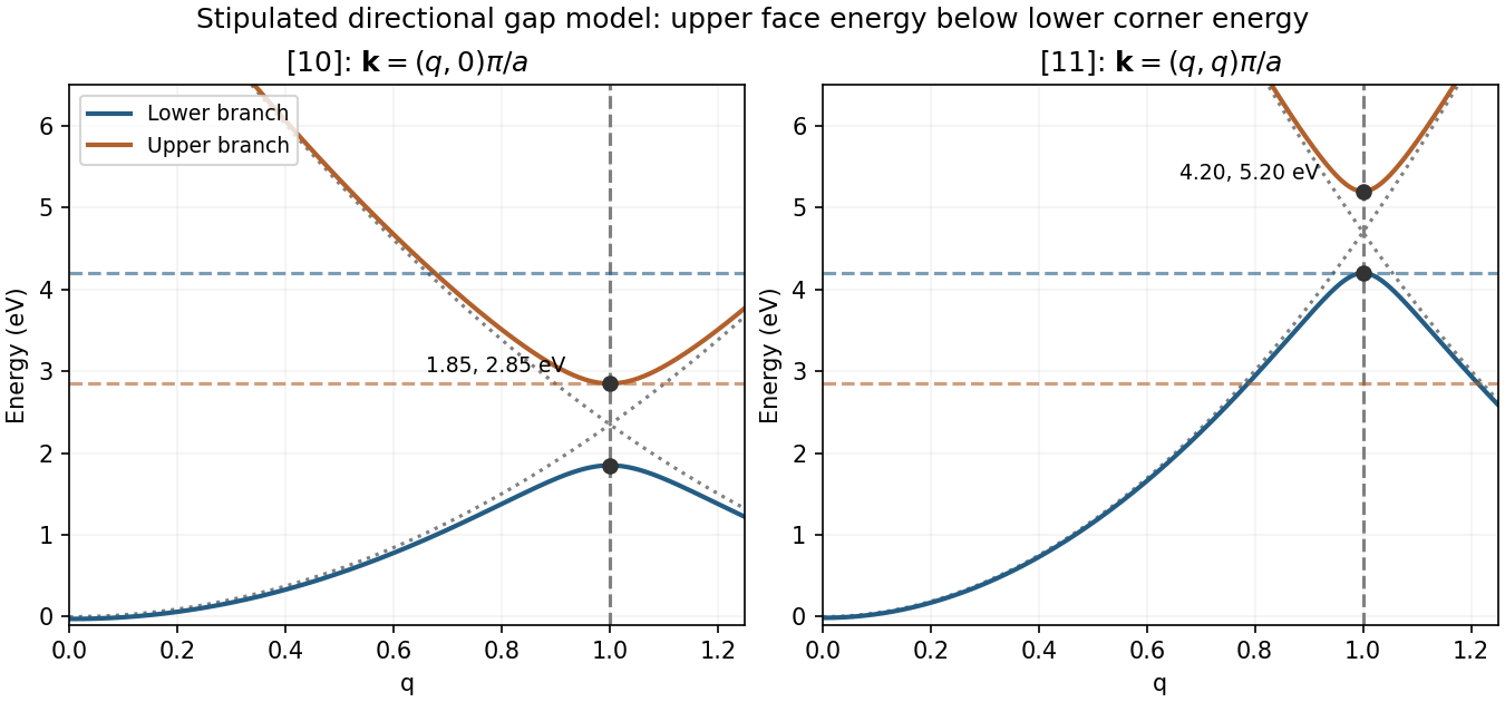
Original directional avoided crossings and the overlap of lower- and upper-band boundary energies
. Details. Past exam of the physics A course of the University of Cambridge 2014 Paper 2 Section C C10 Solution by Codex 0 2026-10-20
Codex 0 2026-10-20The Pauli exclusion principle confines thermally excited conduction electrons to an energy interval of order around the Fermi surface. Their excess energy is therefore proportional to , giving an electronic heat capacity . More precisely, . In a three-dimensional Debye model, acoustic phonons have density of states proportional to ; their thermal energy scales as , givingper mole of atoms. This assumes a normal metal without a lower-temperature superconducting or magnetic anomaly.
For , the lattice approaches the Dulong-Petit value, so , usually dominated by . Each classical vibrational mode contributes through kinetic and potential equipartition. This is a high-temperature solid-state regime, not a claim that the solid persists to arbitrarily high temperature; anharmonicity and can matter.
The body-centred cubic cell has two atoms, so . Counting three acoustic branches gives . By the Debye-temperature definition,This is an effective Debye sound speed; separate longitudinal and transverse speeds are not determined. For isotropic branches, .
Past exam of the physics A course of the University of Cambridge 2014 Paper 2 Section B B9 Solution by Codex 0 2026-10-20
Codex 0 2026-10-20For time dependence , a scalar Fresnel-Kirchhoff aperture formula for a point-source amplitude isHere , , and is the obliquity factor, approximately the mean of the incident and outgoing direction cosines measured with the forward aperture normal. The factors describe incident spherical spreading, outgoing spreading and accumulated phase. This is the scalar Kirchhoff aperture approximation; it does not supply an exact electromagnetic edge boundary solution.
In the Fresnel regime, expand path lengths to quadratic order in aperture coordinates while replacing slowly varying amplitude and obliquity factors by their axial values. In the Fraunhofer regime the quadratic aperture phase is negligible, leaving the aperture Fourier transform. For characteristic aperture size , the latter requires in the relevant finite-source geometry; a lens can supply the Fourier-plane configuration.
For the one-dimensional Cornu construction, put on the unobstructed straight ray, with the aperture plane perpendicular at . An element is displaced transversely by , with , where and . A long straight edge or slit makes the other transverse direction separable. Then
For knife-edge diffraction at the fence, the edge is above the direct ray, with , , , and . The unblocked aperture extends upward from , so its Cornu chord runs from to infinity. Using and normalizing by the full unobstructed chord givesThe approximate chord coordinates are , . This is the standard single-knife-edge Fresnel normalization.[ref]
Propagation by diffraction (ITU-R P.526-13) by International Telecommunication Union. Annex 1, Sections 2.7 and 4.1, Fresnel integrals and single knife edge
For geometric spreading in a moving-receiver diffraction measurement, set while retaining and :Normalized transmission decreases toward the fence. Absolute received intensity initially increases, because the free-space spherical-wave intensity rises as source–receiver distance decreases. In this model it reaches a maximum near , then falls. The formal paraxial small- behavior is ; extrapolation to is outside the small-angle approximation. The sketch distinguishes the absolute signal from its ratio to the unobstructed signal at each position.
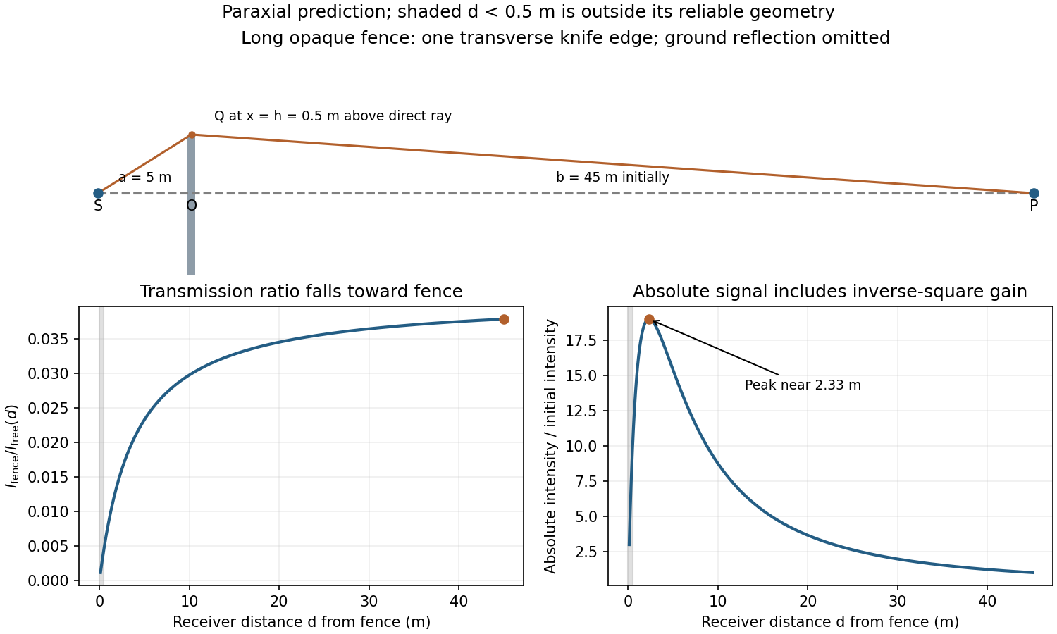
Original knife-edge geometry and distinct absolute-intensity and normalized-transmission predictions
. Details. Pinned article: Introduction to the OurBigBook Project
Welcome to the OurBigBook Project! Our goal is to create the perfect publishing platform for STEM subjects, and get university-level students to write the best free STEM tutorials ever.
Everyone is welcome to create an account and play with the site: ourbigbook.com/go/register. We belive that students themselves can write amazing tutorials, but teachers are welcome too. You can write about anything you want, it doesn't have to be STEM or even educational. Silly test content is very welcome and you won't be penalized in any way. Just keep it legal!
Intro to OurBigBook
. Source. We have two killer features:
- topics: topics group articles by different users with the same title, e.g. here is the topic for the "Fundamental Theorem of Calculus" ourbigbook.com/go/topic/fundamental-theorem-of-calculusArticles of different users are sorted by upvote within each article page. This feature is a bit like:
- a Wikipedia where each user can have their own version of each article
- a Q&A website like Stack Overflow, where multiple people can give their views on a given topic, and the best ones are sorted by upvote. Except you don't need to wait for someone to ask first, and any topic goes, no matter how narrow or broad
This feature makes it possible for readers to find better explanations of any topic created by other writers. And it allows writers to create an explanation in a place that readers might actually find it.
Figure 1. Screenshot of the "Derivative" topic page. View it live at: ourbigbook.com/go/topic/derivativeVideo 2. OurBigBook Web topics demo. Source. - local editing: you can store all your personal knowledge base content locally in a plaintext markup format that can be edited locally and published either:This way you can be sure that even if OurBigBook.com were to go down one day (which we have no plans to do as it is quite cheap to host!), your content will still be perfectly readable as a static site.
- to OurBigBook.com to get awesome multi-user features like topics and likes
- as HTML files to a static website, which you can host yourself for free on many external providers like GitHub Pages, and remain in full control

Figure 2. You can publish local OurBigBook lightweight markup files to either OurBigBook.com or as a static website.
Figure 3. Visual Studio Code extension installation.
Figure 5. . You can also edit articles on the Web editor without installing anything locally. Video 3. Edit locally and publish demo. Source. This shows editing OurBigBook Markup and publishing it using the Visual Studio Code extension. 
- Infinitely deep tables of contents:




All our software is open source and hosted at: github.com/ourbigbook/ourbigbook
Further documentation can be found at: docs.ourbigbook.com
Feel free to reach our to us for any help or suggestions: docs.ourbigbook.com/#contact