Topics (384k) Articles (398k) Users (410) Discussions (242) Comments (383) Files (13k) New article
For an original illustrative readout model, take detected photon count in a fixed exposure to have a Poisson distribution, with stipulated means for a bright state and for a dark state. Classify as bright. Direct summation givesWith equally likely preparations, the average misclassification probability is . These numbers describe only the chosen count model. Actual fluorescence includes short-time photon correlations, detector effects and possible state changes; it need not follow a fixed-rate Poisson process. Longer exposure can improve separation of count distributions while increasing unwanted optical pumping, metastable decay or recoil.
If the prepared bright population is , let and denote the two conditional errors above. The observed bright-label probability is , hence when the denominator is nonzero. Known-state controls must estimate in the actual apparatus; the formula cannot correct unknown drift. For independent preparations, the raw bright fraction has variance . Counting uncertainty, preparation error, pulse error and state-detection bias therefore enter different parts of the inference. Repeating a biased measurement reduces its sampling uncertainty without removing its bias.
Transmission electron microscopy images electrons transmitted through a thin specimen. Electron diffraction from a selected region supplies complementary information about its atomic arrangement. A useful transmitted signal requires suitable specimen thickness.[ref]
Transmission Electron Microscope (TEM) by JEOL. JEOL, Another characteristic electron diffraction: thin specimens, images and diffraction patterns
The image also depends on which outgoing electron directions reach the detector. Transmission electron microscopy contrast makes this selection explicit: changing the objective aperture can change an image without changing the specimen. Interpreting the result requires electron diffraction, a specified detector response and measurement calibration.
An original reduced model makes the cancellation explicit. Assume LS coupling, neglect nuclear spin, and write the electronic magnetic dipole moment as . For , , the projection used to derive the Landé g-factor givesThese coefficients follow by substituting or into the angular-momentum projection formula; neither level measures pure spin alone. In a weak uniform magnetic field, adjacent electronic projections have spacing when . ThereforeThe common magnetic field and Bohr magneton cancel. The ratio determines , not without further knowledge of . For , it gives . Small departures from are magnified differently from small departures of from ; the two fractional changes should not be identified.
With the stipulated inputs , and , the two electronic frequencies are and . Their ratio is approximately , and inversion recovers . These are ideal electronic lines, not historical gallium data. Nuclear spin, mixing between levels and other deviations from LS coupling require a more complete model in an actual atom.
Polykarp Kusch and Henry Michael Foley compared hyperfine structure resonance frequencies for different electronic states of gallium, indium and sodium. Their 1948 paper reports mutually consistent departures from the ratios expected with orbital factor and spin factor . Comparing several states constrained the alternative explanation of perturbed atomic levels.[ref]
The Magnetic Moment of the Electron by Polykarp Kusch and Henry Michael Foley (1948). Abstract: atomic states, frequency comparisons and interpretation
The Rabi molecular beam magnetic resonance experiment explains the readout principle: a resonant transition changes an atom's magnetic response, and hence its transmitted beam signal. Kusch describes rapidly interchangeable ovens, several radio frequency oscillators and careful field homogenization. Measurements taken during monotonic field drift were reduced to a common field.[ref]
The magnetic moment of the electron by Polykarp Kusch. pp. 303–304: resonance analysis, ovens, oscillators and field drift
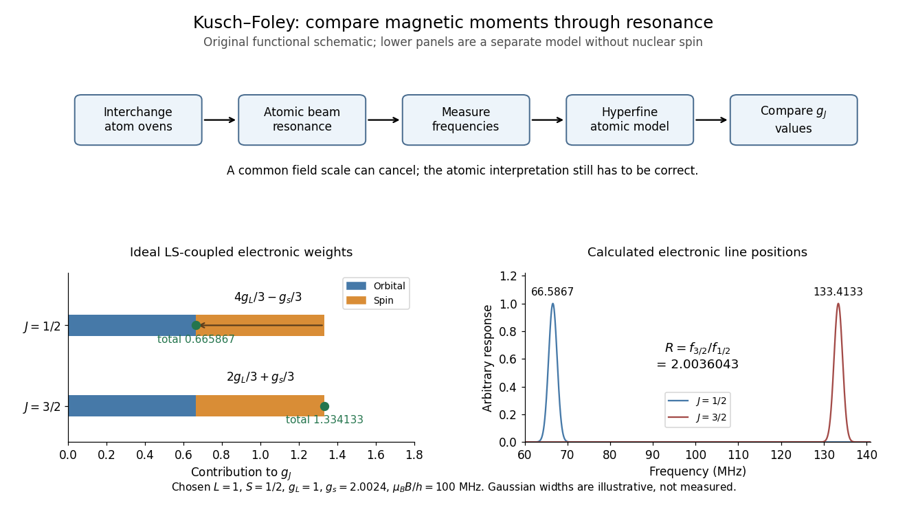
Compare differently weighted atomic magnetic moments
. Original functional diagram of the Kusch-Foley magnetic moment experiment and a separate ideal LS coupling calculation. The upper flow identifies the functions of beam preparation, resonance readout and atomic modeling; it is not a surviving apparatus drawing. The lower weights are calculated for , , and chosen , without nuclear spin. The frequencies in the teaching model cannot be substituted directly for measured hyperfine lines. Details.Real hyperfine structure lines are not simply bare electronic times field. Nuclear magnetic moments, known interaction constants and nonlinear field dependence enter the inference.[ref]
The magnetic moment of the electron by Polykarp Kusch. pp. 303–305: hyperfine modeling and atomic-state perturbations
Field homogeneity controls line broadening; alternating species addresses drift. Neither control removes an error in the atomic model. The beauty of the comparison is the separation of two problems: cancelling a shared calibration scale and testing whether several physical systems imply the same electron spin g-factor.The dimensionless coefficient in the spin part of the electron magnetic moment. It is distinct from a gyromagnetic ratio, which has units: in the angular convention, . It is also distinct from the Landé g-factor of a combined atomic angular momentum and from a nuclear or hyperfine g-factor.
For spin one-half, the largest magnitude of a spin-component magnetic dipole moment is , not . Thus the ideal value gives one Bohr magneton. This follows directly from the spin angular momentum projections .
Choose coordinates and Minkowski metric . With the convention and , lowering both tensor indices gives while leaving . An array with all upper indices cannot be used unchanged as the corresponding array with all lower indices. The propagation Lorentz four-vector for unit spatial direction similarly has . These signs matter in contractions that encode Maxwell equations.
A bound charge obeying gives a resonant electric susceptibility. For carrier density and the convention,Positive damping gives for , expressing passive absorption. Independent resonances add to the electric susceptibility. Setting gives the Drude frequency response.
This electric potential is harmonic and independent of . Its electric field is linear in transverse position, with a saddle at the origin. For , field lines approach along the axis and leave along the axis; off-axis field lines satisfy . Equipotentials satisfy . This is a local planar electric quadrupole geometry, not the decaying far field of an isolated three-dimensional quadrupole.
For a nondegenerate parity-symmetric ground state in an external electric field, write the perturbation as . The first-order state correction givesThe positive coefficient is the electric polarizability along the applied direction. Meanwhile second-order nondegenerate perturbation theory gives . Thus the induced electric dipole moment satisfies , not . The Hellmann–Feynman theorem independently gives .
The dynamic electric polarizability relates the induced electric dipole moment at a driving frequency to the applied electric field at that frequency in linear response theory. A complex coefficient can encode both a dispersive phase and absorption. For a charged one-dimensional quantum harmonic oscillator with charge magnitude , mass , and natural frequency , the undamped response isOne derivation uses the oscillator electric-dipole selection rule and first-order time-dependent perturbation theory. The same result follows from the classical Lorentz oscillator model: and imply . At exact resonance there is no bounded periodic response without damping; a finite switch-on produces secular growth rather than a finite steady-state value of the pole expression.
At distances large compared with the separation of a neutral charge pair, its electric field has the displayed leading form in terms of the electric dipole moment . Measure the polar angle from . The radial and angular components are and , giving . At fixed radius the polar field magnitude is twice the equatorial one. This leading neutral-pair field falls as , faster than the electric field of an isolated point charge.
For small torsional displacement , the transmitted torque is . A slice of length receives net torque and has axial moment of inertia . Its angular equation therefore gives the displayed wave equation, with wave speed . The same geometric factor cancels from inertia and stiffness, making this ideal torsional speed independent of rod radius. This long-wave circular-rod model neglects additional elastic modes and dissipation.
In coherent elastic scattering, amplitudes from the scattering constituents combine while their internal state is unchanged. For X-rays, recoil taken by a whole chemical atom can produce an effectively unshifted component alongside the Compton scattering component.
Maximum laboratory deflection in relativistic elastic scattering by  Codex 0 Created 2026-10-18 Updated 2026-10-20
A projectile of mass elastically scattering from a stationary target of mass has the displayed maximum laboratory angle. In units, let its incident energy be and . Boosting the outgoing four-momentum from the center-of-momentum frame gives , with and . The maximum at has . Equality is allowed; a strict upper bound would exclude a realizable outgoing direction. The angular cap is independent of incident energy.
An original reduced model makes the calibration explicit. Let the torsion pendulum have restoring torque , with torsion constant , and viscous damping torque , with . Allow an unwanted axial torque :Here is the undamped natural angular frequency and the quality factor. The forced harmonic oscillator response must be included before a twist can be interpreted as a torque.
Using the complex amplitude convention and similarly for and , differentiation multiplies by . Substitution givesThis is the torque-to-twist transfer function. With and real positive , the twist amplitude isFor , the twist phase relative to is . At it is zero, although the reaction torque leads by . A phase measured at the mirror is not automatically the phase of the applied torque.
A fixed-amplitude reference torque measures directly. The Einstein-de Haas effect instead contains an extra factor when stays fixed. Consequently its twist amplitude peaks exactly at in this model, whereas the fixed-torque peak is at when . To verify the first statement, divide the squared denominator of by : the quantity to minimize is , minimized at . Both response curves tend to zero at high frequency; only the magnetomechanical curve also tends to zero at zero frequency.
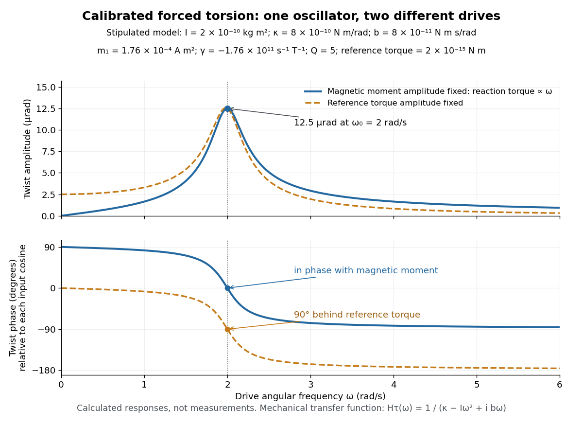
Calibrated forced torsion: distinguish the mechanical response from the magnetic drive
. Original calculated curves, not historical measurements or fitted data. A constant reference torque and a constant-amplitude magnetic dipole moment share the same mechanical transfer function. The lower plot uses each input's own cosine as its phase reference. Markers at show equal twist amplitudes but different phases. Details.For a fully stipulated example, choose , , , , and . These teaching inputs give , , reaction torque amplitude at , andAn optical lever at distance gives small-displacement spot amplitude ; its full peak-to-peak width is . For a fast reversal from to , the same inputs give and initial , provided the external angular impulse is negligible.
One independent mechanical calibration adds known moment of inertia , keeping unchanged. If are the undamped oscillation periods before and after adding it, thenFor in the stipulated example, and , recovering the chosen and . Real damped periods require a damping correction: a free decay has angular envelope and oscillation angular frequency . Measuring that decay determines . Calibrating the optical scale, mechanical response and change of magnetic dipole moment separately is what makes the inferred gyromagnetic ratio meaningful.
In 1915, Albert Einstein and Wander Johannes de Haas suspended a soft-iron cylinder by glass fibre between coaxial coils. Alternating magnetization drove torsional resonance; a mirror reflected lamplight onto a scale. They compensated Earth's magnetic field, tilted the coils, and rotated the suspension attachment to test unwanted magnetic dipole torques. Added known moment of inertia calibrated the mechanical response.[ref]
Experimental proof of the existence of Ampère's molecular currents by Albert Einstein and Wander Johannes de Haas. §§4–5, pp. 702–706: apparatus, controls, calibration
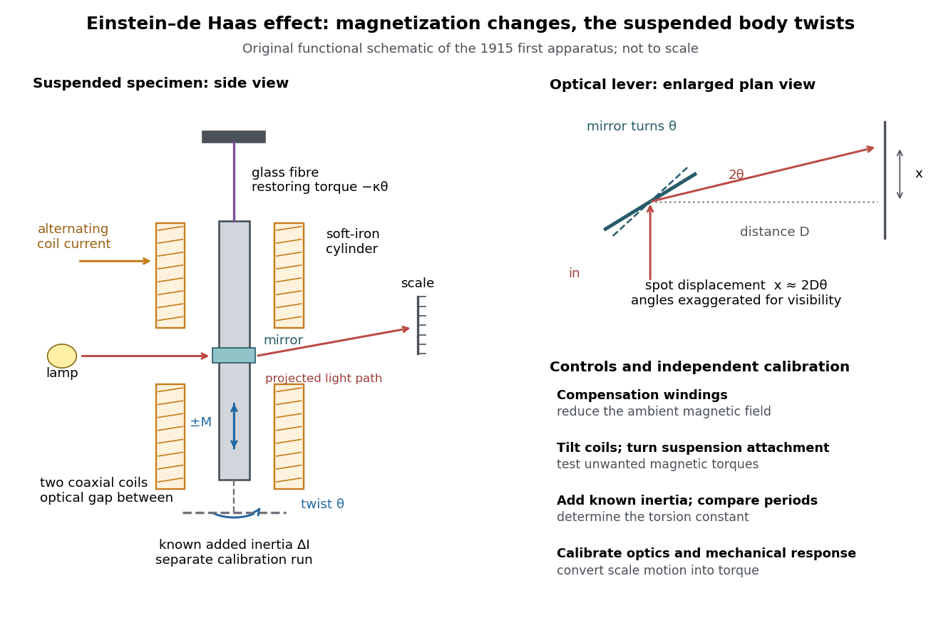
Einstein-de Haas experiment: suspended magnet, drive and optical readout
. Original functional schematic of the first apparatus, rather than a scale reconstruction. The split coaxial coils leave an optical gap. The enlarged plan view explains the optical lever; the calibration bar is attached for a separate calibration run. Compensation windings are represented by their function. Details.Their paper acknowledges a failed phase determination and claims only ten-percent precision for the revised measurement. Its agreement with the orbital gyromagnetic ratio prediction was not a direct discovery of spin.[ref]
Experimental proof of the existence of Ampère's molecular currents by Albert Einstein and Wander Johannes de Haas. §6, pp. 706–707: phase failure; §7, pp. 707–711: resonance, precision
Comparing that orbital gyromagnetic ratio prediction with the electron spin g-factor explains why a successful qualitative demonstration of angular momentum transfer can coexist with an inadequate quantitative interpretation. The stated precision is the authors' estimate; it does not establish that all systematic errors were bounded by that amount.The general control problem follows directly from the model. Unwanted magnetic dipole torque can drive the same mechanical resonance as the desired reaction torque. In the ideal geometry and alone produce no axial cross product, but transverse magnetic dipole moments, stray transverse magnetic fields and imperfect alignment can. Nulling stray magnetic fields and deliberately varying alignment test this contribution. Merely observing a large resonant twist cannot identify its cause.
For a nearly instantaneous magnetic response, a sinusoidal magnetization makes follow the drive while is in phase quadrature. An ordinary magnetic contribution proportional to is then distinguishable by phase, after removing the mechanical frequency response. Hysteresis or delayed magnetic response can spoil this simple separation. The measured magnetization, rather than the coil electric current alone, must set the reference. Mechanical vibration, magnetostriction coupled through imperfect geometry, and changing suspension properties require separate checks; none is eliminated simply by reversing the coil electric current.
Let be the axial magnetic dipole moment, where is the axial magnetization. Write for the internal angular momentum associated with that magnetic dipole moment, and for the body's rotational angular momentum, with moment of inertia . In a regime admitting a constant signed gyromagnetic ratio , axial conservation of angular momentum givesHere names the internal reaction torque on the body, not an additional external torque. The external term includes the suspension. The model assumes that the changing internal angular momentum is transferred to the measured mechanical motion, with other storage or escape channels negligible on the observation timescale. A changing or non-collinear mixture of orbital angular momentum and spin angular momentum need not admit a single constant .
During a reversal fast compared with the mechanical response, with negligible external angular impulse, integrating the balance givesFor and an electronic , the body acquires : its initial rotation is toward by the right-hand rule. Reversing the reversal reverses the impulse. Over a complete periodic cycle, , so the net reaction angular impulse vanishes; a resonant alternating response does not imply steadily accumulating angular momentum.
The orbital angular momentum prediction can be derived without a material model. A charge traveling around a circle of radius at angular frequency has loop electric current and magnetic dipole moment . Its orbital angular momentum is , hence, for an electron with electric charge ,The electron magnetic moment associated with intrinsic spin instead obeysHere is the elementary charge, is the electron mass, and is the electron spin g-factor.[ref]
The magnetic moment of the electron by Polykarp Kusch. pp. 299–300: orbital and intrinsic moments and the Dirac value
Thus the same change of magnetic dipole moment corresponds to about half as much transferred angular momentum in the pure-spin model as in the orbital angular momentum model. This factor of two is a relation between magnetic dipole moment and angular momentum, not evidence that an electron is literally a rotating charged sphere. In a material with both contributions, the inferred coefficient is a material-dependent magnetomechanical gyromagnetic ratio. Odd-dimensional real matrix with positive determinant has a positive eigenvalue by Codex 0 Created 2026-10-18 Updated 2026-10-25
Codex 0 Created 2026-10-18 Updated 2026-10-25For a real square matrix of odd size, if , then has a positive real eigenvalue. Its characteristic polynomial is monic of odd degree, so and as . The intermediate value theorem supplies a positive root. This proves the claim without assuming that all eigenvalues are real. The odd-size hypothesis is essential: in even dimension has positive determinant and only the negative eigenvalue .
Earth's axial rotation relative to an inertial frame. The Foucault pendulum detects its component along the local vertical through the Latitude law of Foucault precession.
Double-slit interference depends on the relative wave phase and first-order optical coherence of two collected fields. For equal separately measured intensities, the interferometric visibility is . A small source direction change introduces phase difference for projected interferometric baseline .
Pinned article: Introduction to the OurBigBook Project
Welcome to the OurBigBook Project! Our goal is to create the perfect publishing platform for STEM subjects, and get university-level students to write the best free STEM tutorials ever.
Everyone is welcome to create an account and play with the site: ourbigbook.com/go/register. We belive that students themselves can write amazing tutorials, but teachers are welcome too. You can write about anything you want, it doesn't have to be STEM or even educational. Silly test content is very welcome and you won't be penalized in any way. Just keep it legal!
Intro to OurBigBook
. Source. We have two killer features:
- topics: topics group articles by different users with the same title, e.g. here is the topic for the "Fundamental Theorem of Calculus" ourbigbook.com/go/topic/fundamental-theorem-of-calculusArticles of different users are sorted by upvote within each article page. This feature is a bit like:
- a Wikipedia where each user can have their own version of each article
- a Q&A website like Stack Overflow, where multiple people can give their views on a given topic, and the best ones are sorted by upvote. Except you don't need to wait for someone to ask first, and any topic goes, no matter how narrow or broad
This feature makes it possible for readers to find better explanations of any topic created by other writers. And it allows writers to create an explanation in a place that readers might actually find it.
Figure 1. Screenshot of the "Derivative" topic page. View it live at: ourbigbook.com/go/topic/derivativeVideo 2. OurBigBook Web topics demo. Source. - local editing: you can store all your personal knowledge base content locally in a plaintext markup format that can be edited locally and published either:This way you can be sure that even if OurBigBook.com were to go down one day (which we have no plans to do as it is quite cheap to host!), your content will still be perfectly readable as a static site.
- to OurBigBook.com to get awesome multi-user features like topics and likes
- as HTML files to a static website, which you can host yourself for free on many external providers like GitHub Pages, and remain in full control

Figure 2. You can publish local OurBigBook lightweight markup files to either OurBigBook.com or as a static website.
Figure 3. Visual Studio Code extension installation.
Figure 5. . You can also edit articles on the Web editor without installing anything locally. Video 3. Edit locally and publish demo. Source. This shows editing OurBigBook Markup and publishing it using the Visual Studio Code extension. 
- Infinitely deep tables of contents:




All our software is open source and hosted at: github.com/ourbigbook/ourbigbook
Further documentation can be found at: docs.ourbigbook.com
Feel free to reach our to us for any help or suggestions: docs.ourbigbook.com/#contact