
Concave function Created 2026-09-24 Updated 2026-10-14
Convex function Created 2026-09-24 Updated 2026-10-14
A function on a convex set is a convex function if, for every and ,Geometrically, a line segment joining two points of its graph of a function lies on or above that graph of a function. The convex set condition ensures that the intermediate input stays in the domain of a function. An affine function satisfies the defining inequality with equality.
For the quadratic function , the inputs and have equally weighted arithmetic mean . Evaluating at the arithmetic mean gives , whereas averaging the outputs gives . Averaging first saves one unit in this example. More generally, direct expansion givesThis identity proves convexity and also shows exactly when its defining inequality is strict.
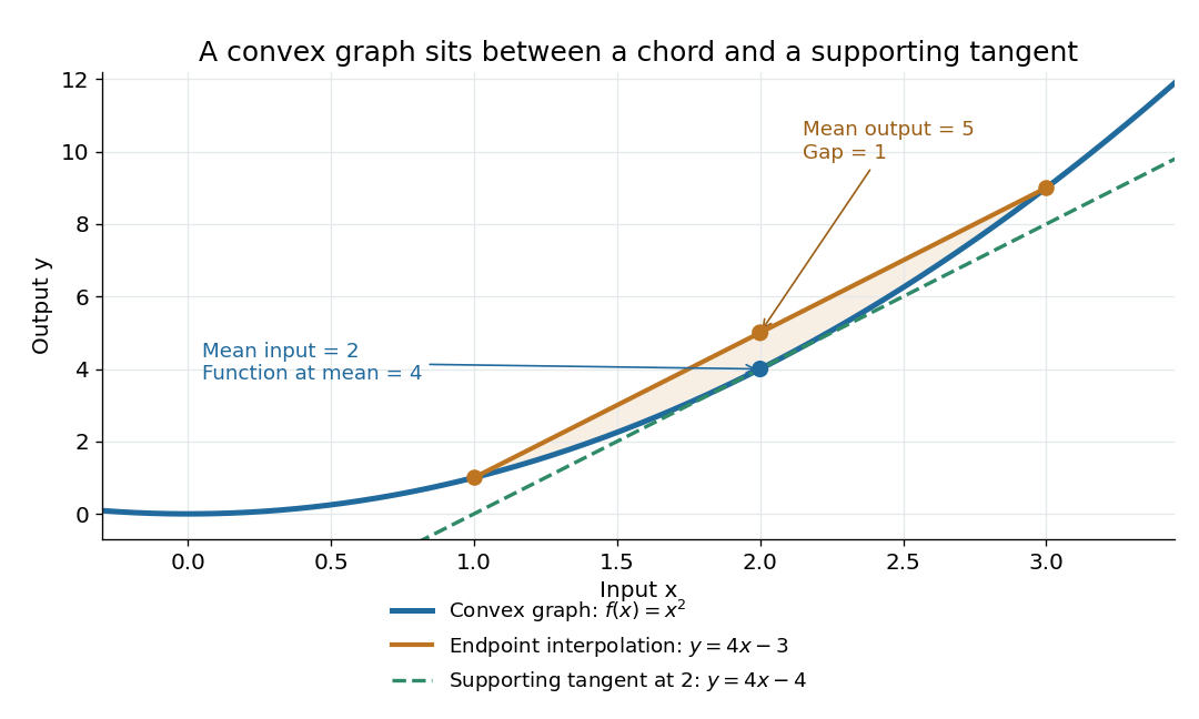
The graph of a convex quadratic lies below its endpoint interpolation and above its supporting tangent
. For , the line segment through and has height at , while the graph of a function has height . The tangent line is an affine minorant: everywhere. Details.For a differentiable convex function, the tangent line in one dimension, or the corresponding supporting affine function in several dimensions, lies below the entire graph of a function. This is the subgradient inequality. The equivalent geometric statement is that the epigraph, consisting of points on or above the graph of a function, is a convex set. These characterizations are developed in Boyd and Vandenberghe's convex-function slides, sections 3.1–3.4.
Convexity does not require differentiability: the absolute value function is a convex function with a corner at . When a function is twice continuously differentiable on an open interval, it is a convex function exactly when its second derivative is nonnegative throughout that interval. In several dimensions, the corresponding criterion on an open convex set is that its Hessian matrix is positive semidefinite everywhere. The domain of a function matters: is a convex function on , but not on all of . A strictly positive second derivative is sufficient for strict convexity, but is not necessary: is a strictly convex function although its second derivative vanishes at .
The usefulness of convexity is that local information can certify a global conclusion. Every local minimum of a convex function on a convex set is a global minimum: if a lower value existed elsewhere, the defining inequality would produce lower values arbitrarily close to the proposed local minimum. For a differentiable convex function on an open convex set, a zero gradient therefore certifies a global minimum. Strict convexity gives uniqueness when a global minimum exists; it does not supply existence by itself. These facts explain the role of convex functions in convex optimization.
Convergent subsequence Created 2026-09-24 Updated 2026-10-14
A convergent subsequence of is a sequence with strictly increasing indices that converges to a limit.
Infimum Created 2026-09-24 Updated 2026-10-14
For a nonempty set , a real number is its infimum precisely when it is a lower bound and every other lower bound is at most . It is the greatest lower bound, not necessarily the minimum.
For , zero is a lower bound. Every positive candidate fails: the Archimedean property gives an integer , hence . Thus , although zero is never a member of . This is the lower-edge counterpart of approximating an unattained supremum.
Supremum Created 2026-09-24 Updated 2026-10-14
For a nonempty set , a real number is its supremum precisely when it is an upper bound and no smaller real number is an upper bound. It is unique: two least upper bounds must each be no greater than the other.
For , every number at least one is an upper bound, and none smaller than one bounds the whole set. Thus , although . For , that same supremum is also the maximum. The approximation property of a supremum supplies witnesses arbitrarily close to an unattained upper edge.
Riemann integration Created 2026-09-24 Updated 2026-11-05
Riemann integration defines an integral by requiring that every sufficiently fine tagged Riemann sum approximate the same number. For a bounded function , a partition of an interval and tags giveThe mesh of a partition must tend to zero, and the answer must be independent of the tags and the chosen partitions of an interval. The equivalent Darboux sum formulation traps every Riemann sum between a lower Darboux sum and an upper Darboux sum. Their common limiting value, when it exists, is the Riemann integral.[ref]
For on , equal-width partitions of an interval give lower and upper values , so the Riemann integral is . For the Dirichlet function, every nondegenerate subinterval has infimum zero and supremum one: lower and upper values remain zero and one. Refining the partition of an interval cannot resolve that gap. Thus boundedness alone does not ensure Riemann integrability; the oscillation of a function on an interval must become small in the weighted aggregate.
Calculus Created 2026-09-24 Updated 2026-10-18
Calculus connects local change with accumulated change. A derivative asks how fast a function changes near one input; an integral adds its contributions across an interval. The fundamental theorem of calculus explains why these operations fit together: accumulating a continuous rate produces a quantity whose derivative is that rate.
For example, suppose a particle moves along a straight line with position metres at time seconds. Its velocity is metres per second. Between and , adding the velocity over time givesHere the velocity stays positive, so the displacement also equals the distance travelled. If the particle reverses direction, the integral of its signed velocity still gives displacement, while the integral of its speed gives total distance.
This is useful because local rules are often easier to specify than whole trajectories. A differential equation can prescribe a particle's velocity or a population's growth rate; integration then reconstructs its evolution, subject to an initial condition. In the other direction, a derivative extracts local information from a known function, and optimization uses that information to locate or approach promising inputs. The same two operations therefore connect measurement, prediction and design.
The visual connection is developed in derivative, integral and fundamental theorem of calculus. The definitions depend on limits, which turn progressively finer finite measurements into exact mathematical statements. A graph with a corner need not have a derivative there, and the conditions permitting integration or interchange of limits matter; calculus is more than a collection of symbolic rules.
Historically, Isaac Newton described changing quantities and their rates in the language of fluents and fluxions; his manuscript History of the Method of Fluxions records that approach.[ref]
https://www.newtonproject.ox.ac.uk/view/texts/normalized/NATP00356. Isaac Newton, History of the Method of Fluxions, Cambridge University Library MS Add. 3968
Gottfried Wilhelm Leibniz's Nova methodus pro maximis et minimis appeared in Acta Eruditorum in October 1684, pp. 467–473; the original article is preserved in the HKUST Library collection.[ref]https://digitalcollections.hkust.edu.hk/Detail/objects/b540295. Gottfried Wilhelm Leibniz, Nova methodus pro maximis et minimis, 1684
The modern limit definitions used here should not be read back into those seventeenth-century formulations. Sequence and series Created 2026-09-24 Updated 2026-11-05
A sequence is an ordered family , formally a function from the positive integers into a chosen set. The indices record position and allow repeated values. A series formed from that sequence studies the partial sumsWriting means that the sequence has finite limit . Thus convergence of terms and convergence of their cumulative sums are different assertions.
For , the terms tend to zero and the geometric series has . For , the terms also tend to zero, but the harmonic series diverges. A necessary condition for series convergence follows from ; it is not sufficient. The Cauchy criterion for series instead controls every sufficiently late finite tail.
For a sequence of functions, there are two further choices: pointwise convergence checks a separate limit at each input, while uniform convergence requires a common error bound over the domain. These distinctions determine when infinite sums may be integrated or differentiated.
Lp norm Created 2026-09-24 Updated 2026-10-14
An Lp norm measures the size of a measurable function by averaging a power of its absolute value with respect to a specified measure. For ,when the integral is finite. The exponent controls how strongly large values influence the result. The Lp space identifies functions equal almost everywhere, so this becomes a norm on the corresponding equivalence classes. For , use the essential supremum of , as defined by the L-infinity norm. [ref]
Lp spaces (Chapter 7 of Measure Theory). Hunter, Measure Theory, Definitions 7.1 and 7.4: Lp spaces and norms
.For a two-coordinate vector , treat the coordinates as a function on two inputs with counting measure. Then , , and . The middle case is the Euclidean norm; the first adds the coordinate magnitudes, and the last takes their largest value. These are different answers to different questions about size, all satisfying the triangle inequality.
If instead each input has probability , the same values give and , while remains unchanged. Thus the measure is not an optional label. On a probability space, the finite Lp norms are nondecreasing in whenever they are finite, by Hölder's inequality; the unnormalized two-coordinate example above decreases instead. Statements comparing different exponents must specify their measure convention.
Why are these sizes useful? If is an error function, its L1 norm measures aggregate absolute error, its L2 norm measures the square root of aggregate quadratic loss, and its L-infinity norm bounds error almost everywhere. Concentrating a large error on a set of small positive measure can give a modest finite Lp norm but a large L-infinity norm. The three-point example and diagram in L-infinity norm show this explicitly, including why a null set behaves differently from a rare event.
Coercive function Created 2026-09-24 Updated 2026-10-14
A real-valued function on a normed vector space is coercive when its value tends to positive infinity as the norm of its argument tends to infinity. A continuous coercive function on a finite-dimensional real vector space attains a global minimum.
Extreme value theorem Created 2026-09-24 Updated 2026-10-14
A real-valued function that is continuous on a nonempty compact space attains both a global minimum and a global maximum. In particular, for a continuous function on a nonempty closed interval, there are points such thatThe important word is “attains”: the best values occur at actual allowed inputs, rather than merely being approached. The interval version is [ref].
For a worked example, take on . Its global minimum is , and its global maximum is . Nonnegativity gives the first answer; on the specified closed interval gives the second. The endpoint is essential: looking only for a zero derivative would find the minimum and miss the maximum.
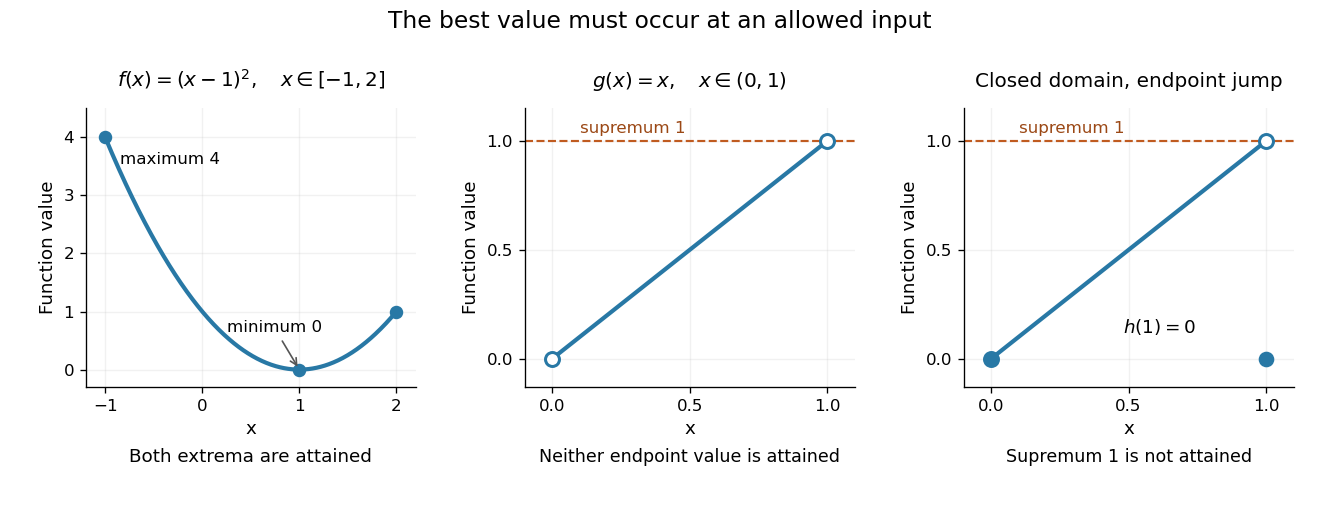
An attained minimum and maximum on a closed interval, compared with excluded endpoints and a discontinuous endpoint value
. Details. For comparison, the continuous function on the open interval has infimum and supremum , but neither is a value of . Even a closed domain is insufficient without continuity: define for , and . On , its supremum is , approached by for , but every function value is strictly less than . This endpoint change makes discontinuous, preventing attainment. On the unbounded real line, the continuous function has neither a global minimum nor a global maximum. These examples show what can fail when a hypothesis is dropped; functions outside the hypotheses may still have extrema.
The extreme value theorem is an existence tool for optimization: first establish that a continuous objective function on a nonempty compact feasible set has a best value, then investigate where it occurs. It neither locates the optimizing point nor promises uniqueness or differentiability. For example, the absolute value function on has its global minimum at zero although no derivative exists there; a constant function has every input as a minimizer. This role in optimization is explained in University of Toronto MAT237 notes, section 1.4: compactness and the extreme value theorem.
A short proof outline identifies the mechanism. The continuous image of a compact space is compact; a nonempty compact subset of the real line contains its infimum and supremum. For a closed interval, one can instead choose inputs whose outputs approach the supremum, extract a convergent subsequence by the Bolzano-Weierstrass theorem, and use continuity to make its limiting output equal that supremum. The closed interval retains the limiting input. Repeating the argument for the infimum supplies the minimum.
Real line Created 2026-09-24 Updated 2026-09-24
Big O notation Created 2026-09-24 Updated 2026-10-14
The statement as means there are constants and such thatThe same constant must work for all sufficiently large inputs. Near a finite limit point , replace by within the domain. Absolute values allow signed or complex-valued functions; when discussing nonnegative operation counts they can be omitted.
The notation records an upper bound, not an exact leading coefficient or necessarily a tight growth order. For example, because for it is at most . It is also , a weaker statement. A tight comparison uses big theta notation; a ratio tending to one uses asymptotic equivalence. Formally denotes a class of functions, and writing is conventional shorthand for membership in that class. [ref]
https://live.ocw.mit.edu/courses/6-006-introduction-to-algorithms-spring-2020/c6d8f06c6f11e3342633dec85498f551_MIT6_006S20_r01.pdf. MIT 6.006, Demaine, Ku and Solomon, Recitation 1, page 3: asymptotic upper and tight bounds
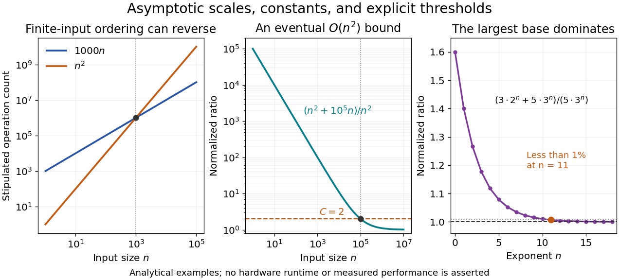


The first panel compares stipulated operation counts and . Although is linear and quadratic, for ; the ordering reverses beyond their crossing. These are mathematical cost models, not measured runtimes. The time complexity notation describes the growth of whichever cost function has been specified, whether that function represents a worst-case bound, an average, or another explicit quantity.
The middle panel gives a concrete eventual bound: for every . Its normalized ratio approaches one, but the threshold matters. The final panel shows the asymptotic comparison of exponential functions, with its geometrically shrinking relative difference.
Constants may depend on fixed parameters. For each fixed , is with ; one constant cannot cover every positive . A uniform big O bound makes this extra quantifier explicit.
The notation was already used in nineteenth-century number theory. In his 1976 paper, Donald E. Knuth reports Landau identifying Bachmann's 1894 book as the first appearance of known to him. Knuth's account gives the earlier mathematical setting of a notation now also common in time complexity analysis. [ref]
https://danluu.com/knuth-big-o.pdf. Knuth, Big Omicron and big Omega and big Theta, 1976, page 19
Lipschitz continuity Created 2026-09-24 Updated 2026-10-14
A function between metric spaces is Lipschitz continuous if one finite number controls every change of output by the corresponding change of input:For real inputs and outputs this is . The same bound must work for every pair in the specified domain of a function. It gives a quantitative version of continuity: an input error of at most produces an output error of at most . The least possible bound is the Lipschitz constant. Lebl presents the real and metric-space definitions and their connection with uniform continuity. [ref]
Three functions show why this condition differs from differentiability. The absolute value has a corner at zero, but the reverse triangle inequality gives , so it has Lipschitz constant one on the real line. The sine is smooth and also has Lipschitz constant one: the mean value theorem and bound every secant slope. The square root is continuous on , butNo finite Lipschitz bound works on that interval. At , the ratios are . Smaller input changes near zero therefore require larger amplification factors.
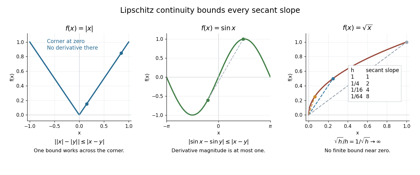
Bounded secant slopes permit a corner, while the square root needs unbounded amplification near zero
. Details. 
For a real function, Lipschitz continuity means that the absolute slopes of all secant lines are bounded. If the derivative exists at a point, taking a limit of those slopes gives . In the other direction, a function that is continuous on a real interval, differentiable in its interior, and satisfies there is Lipschitz continuous by the mean value theorem. The interval hypothesis matters: the theorem uses the segment connecting the two inputs.
A Lipschitz function is uniformly continuous: for , choosing input tolerance works at every point. If , the function is constant. The converse fails; the square root on is uniformly continuous, and satisfies the weaker Hölder continuity bound , without a finite Lipschitz constant. These distinctions are developed in Lebl's worked examples. [ref]
The usefulness is controlled sensitivity. Successive Lipschitz maps with bounds and have a function composition with bound , because each stage amplifies the previous distance by at most its own bound. For an ordinary differential equation, Lipschitz continuity in the unknown state is the condition that makes nearby trial solutions controllably close in the Picard-Lindelöf theorem. For incomplete data, the McShane extension theorem fills in unobserved values while preserving the same bound. This one inequality connects error estimates, uniqueness, and interpolation.
Eventually periodic positional expansion of a rational number Created 2026-09-24 Updated 2026-11-05
A positional expansion in an integer base represents a rational number exactly when its digit sequence is eventually periodic. Long division proves the forward implication because only finitely many remainders occur; summing a periodic tail as a geometric series proves the converse.
Density of the rational numbers Created 2026-09-24 Updated 2026-11-05
Between any two real numbers lies a rational number. By the Archimedean property, choose a positive integer with , and set using the floor function. ThenThis works for negative as well as positive endpoints, because the floor always rounds downward. It proves that the rational numbers are dense in the real line.
There are actually infinitely many rational numbers in each nonempty open interval: after finding one, apply the same argument between that point and the right endpoint, repeatedly. Density concerns the existence of nearby points; it does not say that every real number is rational. In particular, the countable set of rational numbers is dense in an uncountable set.
Rao-Blackwell estimator of a squared normal mean Created 2026-09-24 Updated 2026-11-05
For independent , the unbiased estimator of has mean square error . Conditioning on the Sufficient statistic giveswhose mean square error is .
Euclidean Ramsey set Created 2026-09-24 Updated 2026-09-24
A finite set is Euclidean Ramsey when, for every number of colors, some finite-dimensional Euclidean space has the property that every coloring of it contains a monochromatic isometric copy of .
Monochromatic sums-and-products obstruction Created 2026-09-24 Updated 2026-09-24
There is a finite coloring of the positive integers for which no infinite set has all pairwise sums and pairwise products in one color. Refining this coloring by the parity of the 2-adic valuation also prevents a constant infinite sequence from evading the obstruction.
Hindman theorem Created 2026-09-24 Updated 2026-10-06
Every finite coloring of the positive integers has an infinite sequence for which all nonempty finite sums of distinct terms have one color.
There are unlisted articles, also show them or only show them.