
Work by James D. Jamieson 2026-10-18
Work by Jacques Berthet 2026-10-18
Work by J. Heinrich Matthaei 2026-10-18
Radial tensor moments in three dimensions 2026-10-18
For a radial weight with the required absolutely integrable moments, rotational symmetry makes the second and fourth moments isotropic tensors. The second moment is ; its trace gives . Complete symmetry of the fourth moment forces equal coefficients of the three Kronecker delta pairings. Its double tensor contraction gives , proving the displayed expression. Odd moments vanish under . Choosing to be the indicator function of a spherical shell gives all the corresponding shell moments without separate angular integrations.
For , write and . Integration by parts gives , while . The Cauchy-Schwarz inequality therefore gives the displayed sharp bound, with equality exactly when . A prescribed positive budget consequently givesThis proves the unique global optimum, rather than only stationarity from a Lagrange multiplier.
For a single-valued curve below the chord joining to , with length , the maximum enclosed area is attained by the lower minor circular arc. Equivalently it minimizes at fixed length. Its equation and length areTo prove global minimality for , augment the objective by . The augmented integrand is linear in and strictly convex in . The displayed arc satisfies its Euler-Lagrange equation, so the supporting-line inequality for the convex slope dependence, followed by integration by parts, proves it minimizes the augmented functional among curves with the prescribed endpoints. On the fixed-length class the multiplier term is constant. The semicircle endpoint follows by a limit; its endpoint tangents are vertical but its length is finite.
Gravitational potential producing a circular hanging chain Created 2026-10-18 Updated 2026-10-20
For uniform linear mass density , a chain minimizing at fixed length has Beltrami identity . In the domain , the displayed potential has downward gravitational acceleration . A circular arc satisfies the identity because .
This arc is a global minimum among admissible competitors of the same length with the same endpoints in . Set . The variable part of the energy is , a hyperbolic length in the Poincaré half-plane model. The calibration for semicircular hyperbolic geodesics has . The Cauchy-Schwarz inequality gives , with equality along the circle traversed with increasing . The constant-potential part is unchanged by the fixed-length constraint.
Modeled mitochondrial oxygen traces 2026-10-18
The following original model chooses piecewise constant oxygen consumption rates in a closed, well-mixed suspension. It assumes no gas exchange, negligible addition volume, a corrected sensor and sufficient oxygen throughout. The curves are invented teaching examples, not measured traces, fitted data or a reconstruction of Figure 6.
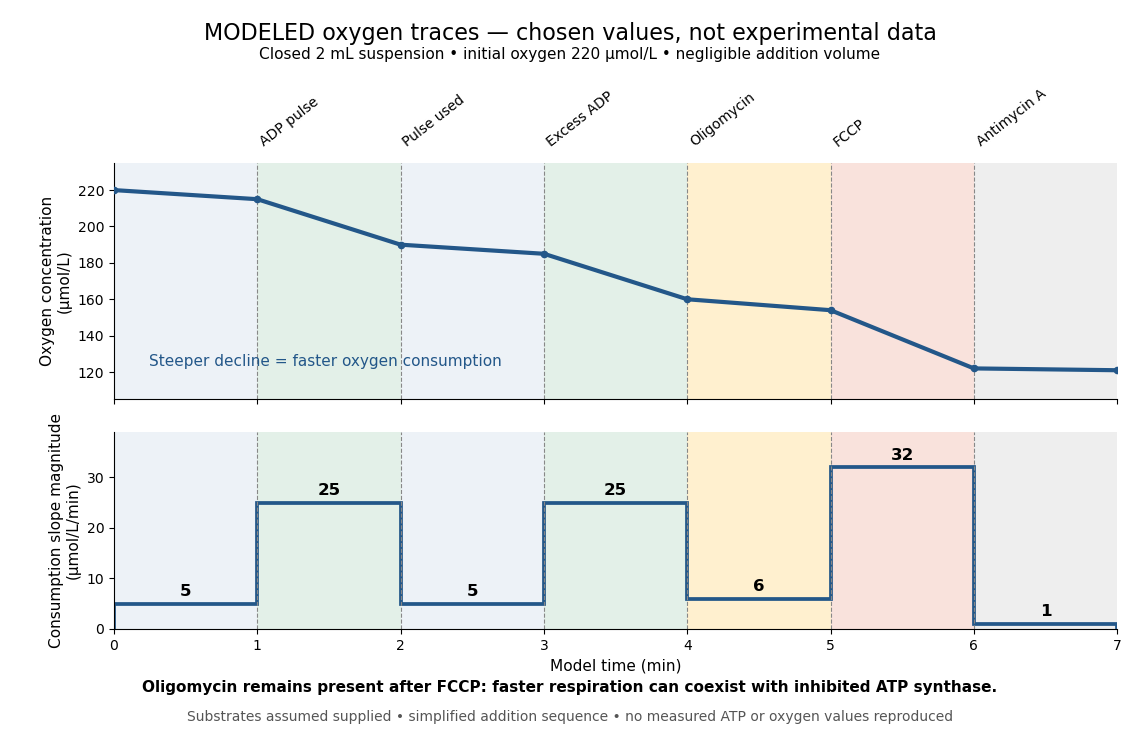

Start at . On successive one-minute intervals, choose positive slope magnitudes . Integration gives the endpoint concentrations . This is just the recurrence , with ; the step plot shows . The trace remains above zero by construction.
During the second ADP interval, the total consumption rate isWith a stipulated mitochondrial protein mass of , that is . Using a denominator twice as large would halve this reported rate without changing the raw oxygen trace. Comparisons therefore need both loading and the chosen denominator.
For a second bookkeeping check, the modeled post-antimycin A slope of corresponds to background. If that background is additive and unchanged in earlier windows, subtraction gives , and for excess ADP, oligomycin and FCCP, respectively. The oligomycin-sensitive difference is . It is a difference in oxygen consumption under the chosen interventions, not an ATP production rate. Converting it into one requires additional coupling assumptions or an independent ATP measurement; the FCCP interval shows why slope alone cannot supply that conversion.
Across the whole seven-minute example, consumption is , also the sum of the seven interval consumptions. This equality checks the rate-to-amount accounting independently of how the intervals are named. Actual records require attention to calibration, mixing transients, background stability and decreasing oxygen availability; a line that steepens or flattens alone does not identify the cause.
Four-spin Ising ring Created 2026-10-18 Updated 2026-10-20
Take a cycle graph with four labeled graph vertices and four distinct edges . Set , , and impose periodic boundary conditions by writing . The square drawing represents a one-dimensional ring: it has no diagonal interactions and is not a two-dimensional lattice.
Call an edge between opposite Ising spins a domain wall. If is their number, the four bond products sum to , so the energy isEach domain wall costs relative to an aligned bond. Returning around the ring must return to the starting Ising spin, so is even: equivalently, . Choosing an even set of wall edges and then choosing determines the entire pattern. The state degeneracy is therefore , using a binomial coefficient.
| Domain walls | State degeneracy | Energy | Total Boltzmann factor weight |
|---|---|---|---|
The twelve middle microstates consist of eight patterns with one exceptional Ising spin and four patterns with two adjacent Ising spins and two adjacent Ising spins. The two alternating patterns have four domain walls. All microstates are shown below.
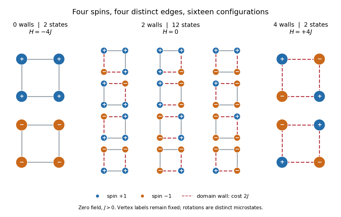

Writing , the partition function and the probability of each energy class areFor an original exact example, choose . Then , , and , , . Each aligned microstate has probability , each middle microstate , and each alternating microstate : multiply by state degeneracy before comparing whole classes. As , all sixteen microstates become equally likely, but the class probabilities approach . As , the two all-aligned microstates each have limiting probability .
Cold-plasma radio dispersion 2026-10-18
Take a cold, unmagnetized, collisionless plasma with uniform equilibrium electron density , fixed neutralizing ions, and a small electromagnetic wave that is a transverse wave. Cold means that thermal-motion corrections are neglected. For electron mass , elementary charge magnitude and electric field , the linear Newton's second law equation is . Thus and the current density is . Writing the induced electric polarization as gives a negative electric susceptibility. With vacuum permittivity ,The plasma frequency controls the response. For , the propagating branch has real refractive index . For , this homogeneous model has an evanescent wave, not an ordinary propagating wave with a negative real refractive index. In a slowly varying vertical profile, a normally incident ray approaches a turning region where ; the geometrical-ray approximation fails right at that region. At oblique incidence the conserved horizontal wave vector changes the turning condition. A smooth density gradient can therefore return a skywave without a mirror or a layer of metal.
For a homogeneous propagating section, direct differentiation of the dispersion relation givesA phase velocity greater than does not send information faster than . Here a narrow wave packet has group velocity , while the full causal response must still respect special relativity. Even this stripped-down plasma is strongly dispersive near its plasma frequency. In the actual ionosphere, collisions produce absorption, and the magnetic field of Earth changes the response with direction and wave polarization; a single real scalar cannot capture all of that behavior.
On 11 December 1924, Edward Victor Appleton and Miles Aylmer Fulton Barnett perform an experiment: the Bournemouth broadcasting radio transmitter slowly changes wavelength; an Oxford radio receiver records alternating maxima and minima from ground wave-skywave wave interference. The inferred equivalent height is about . A separate comparison of simultaneous loop and vertical antenna signals tests the downward arrival direction. The E layer is established first; the higher F layer is found in winter 1926–27. These dates describe different findings.[ref]
The Ionosphere by Edward Victor Appleton. Edward V. Appleton, The ionosphere, Nobel lecture, 12 December 1947, printed pp. 80–81, Fig. 1, Eq. (1), and the wavelength-change and antenna-comparison paragraphs
Why change the wavelength deliberately? Ordinary fading alone could arise from changing emission, receiver drift or a moving propagation path. A controlled sweep predicts a specific progression of phase difference between two arrivals. The directional antenna comparison supplies an independent kind of evidence for an overhead contribution. Agreement supports an atmospheric return; fitting a distance alone would not establish a unique electron density profile. In the model below, comparable received amplitudes make the interference fringes easier to see. A practical repetition would also calibrate the frequency sweep, track radio transmitter output and receiver gain, and compare repeated sweeps with fixed-frequency intervals to detect time drift. These are controls inferred from the measurement model, rather than additional procedures attributed to the historical account.
The radio receiver does not need to resolve two pulses to detect two paths. If one path takes longer, the two contributions reaching the receiver during a slow frequency sweep carry slightly different emission frequencies and can produce a slow beat in the detected amplitude. At strictly fixed frequency with stationary paths, the arrivals instead have a fixed phase difference: there is no continuing beat merely because one path is longer. This distinction connects the historical observation to ionospheric interference fringe spacing.
Skywave 2026-10-18
A skywave is a radio wave returned toward Earth through interaction with the ionosphere. In a smoothly varying plasma, the ray can bend continuously through refraction before returning: there need be no sharp material surface at the apparent point of reflection. Different frequencies, launch directions and wave polarizations can have different paths and losses.
Ground wave 2026-10-18
A ground wave is a radio wave propagating near and along the surface of Earth. In a short-baseline comparison with a skywave, it supplies a reference path. Approximating its distance by the station separation and its speed by the speed of light is a modeling choice; ground properties and frequency can also affect its attenuation and wave phase.
F layer 2026-10-18
The F layer is a higher main region of the ionosphere, above the E layer. Its different electron density and persistence can permit skywave propagation when a probing radio wave passes through the lower E layer.
E layer Created 2026-10-18 Updated 2026-11-05
The E layer is the lower main region of the ionosphere, below the F layer. Its free-electron population is supplied largely by solar ultraviolet photoionization and reduced by recombination. Thus its ordinary daytime ionization rises after sunrise and weakens at night, although sporadic enhancements can occur. Its electron population changes the refractive index experienced by a radio wave.
The Appleton-Barnett radio interference experiment supplied direct evidence for this returning path. On 11 December 1924, Edward Victor Appleton and M. A. F. Barnett varied the transmitted frequency at Bournemouth and observed alternating signal maxima and minima at Oxford. Interference between a ground wave and a skywave gave their path difference, implying an equivalent return height about . Before dawn, reduced E-region ionization later allowed penetration to the higher F layer.[ref]
The Ionosphere by Edward Victor Appleton. Printed pp. 81–84: 1924 interference experiment, upper layer and measured daily ionization variation
This is a frequency-dependent propagation region, rather than a permanent reflecting material wall. The experiment measures an equivalent path height; refraction, collision losses and wave polarization matter when interpreting it in detail.
Quadratic lower bound for a nonsymmetric matrix Created 2026-10-18 Updated 2026-11-05
Let be a real square matrix and suppose for every real vector , with . The Cauchy-Schwarz inequality gives , hence for all . In particular the kernel is zero, so is an invertible matrix. Applying the bound to gives the operator norm estimate in the Euclidean norm.
Symmetry of is unnecessary: for its symmetric part of a matrix . Thus the hypothesis is exactly a positive lower bound on that symmetric matrix, even when the antisymmetric part is nonzero.
Cowan-Reines reactor antineutrino experiment 2026-10-18
Clyde Cowan, Frederick Reines and collaborators tested whether a particle produced by a nuclear reactor could interact again after leaving its source. At Savannah River, water targets containing cadmium chloride lay between liquid scintillators. Opposite detectors recorded prompt positron annihilation gamma rays; Neutron moderation preceded delayed neutron capture signals in cadmium. The arrangement used two target layers and three scintillator layers, with the middle scintillator shared.[ref]
The Neutrino: From Poltergeist to Particle by Frederick Reines. Printed pp. 210–212, Figs. 4–5; individual Washington reproduction
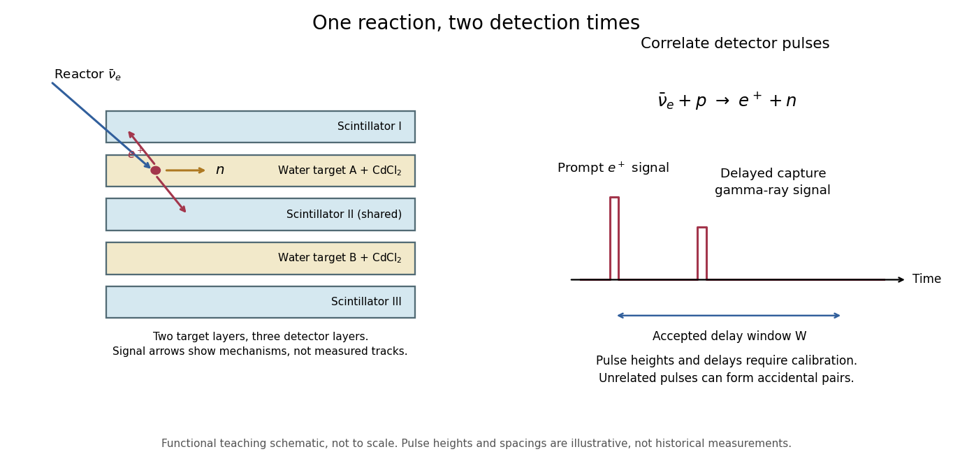
Separate prompt and delayed readouts of an antineutrino interaction
. Details. 
The original functional diagram separates the two signal mechanisms and their timing. It omits dimensions and phototube counts, and is not a reproduction of a historical drawing. The measured objects are detector pulses; identifying their common cause also requires calibration and background tests.
The 1956 paper describes positron-source and neutron-source calibrations, pulse-height gates and photographic pulse records. Diluting the target with heavy water halved the proton density and reactor signal while preserving neutron-detection efficiency. Changing the cadmium concentration altered capture timing; removing it removed the reactor signal. Added shielding tested competing external radiation. These interventions tested the reaction's ingredients, beyond simply observing a reactor-dependent count rate.[ref]
Detection of the Free Neutrino: a Confirmation by Clyde Cowan and others. pp. 103–104, detector analysis and Experimental Results, tests 2–5
Inverse beta decay threshold Created 2026-10-18 Updated 2026-10-20
The neutron and Positron together have more rest mass than the initial proton, so a finite incident energy is necessary even before recoil is considered. In the proton's rest frame, use four-momentum conservation and a negligible neutrino mass. The initial squared center-of-mass energy is ; the least final squared center-of-mass energy is . Equating them gives the threshold above. At threshold the final particles share one center-of-mass velocity; they are not both at rest in the laboratory.
Writing , the result separates intoThe positive second term is the laboratory recoil correction. With rounded rest energies , and , the calculated threshold is about . These rounded inputs follow the recommended particle masses.[ref]
Fundamental Physical Constants — Complete Listing by National Institute of Standards and Technology and others. 2022 CODATA adjustment, proton, neutron and electron mass-energy equivalents in MeV
As a further ideal energy balance, suppose the Positron stops and annihilates with an electron, and all prompt annihilation gamma rays are contained. Its prompt visible energy is . Neglecting neutron recoil gives . Escaping gamma rays, detector response and recoil change that measured sum. The delayed capture signal is a separate energy deposit, not an extra contribution to the incident electron antineutrino's prompt energy reconstruction.
Reciprocal rescaling symmetry of two cross-coupled scalar fields Created 2026-10-18 Updated 2026-11-05
For , the real linear internal transformations preserving the density are and with . There are four connected components; the identity component is the displayed reciprocal rescaling with . In the sum-and-difference basis it preserves a bilinear form of signature , with the identity component isomorphic to that of the One-dimensional Lorentz group. Its Noether current in coordinates is and . The two wave equations give . The energy quadratic form is indefinite: the fields have equal and opposite kinetic signs.
Astronomical interferometer Created 2026-10-18 Updated 2026-11-05
An astronomical interferometer combines observations from separated collecting locations to infer angular source structure. Its projected interferometric baseline determines the angular spatial frequency sampled. Amplitude and intensity interferometers measure different coherence observables; a Michelson stellar interferometer combines optical field amplitudes.
There are unlisted articles, also show them or only show them.