
Paul trap Created 2026-10-18 Updated 2026-10-20
The Paul trap alternates focusing and defocusing electric forces. Their time average along a moving trajectory need not vanish, even when the electric field averages to zero at every fixed point. A spatial gradient makes the fast displacement correlate with the driving electric field; the RF-averaged trapping potential calculates the resulting restoring force.
Wolfgang Paul's lecture describes hyperbolic ring/endcap electrodes, loading by electron-impact ionization of low-pressure gas, and resonant ejection through an endcap hole into an electron multiplier. Sweeping RF voltage produces an air mass spectrum.[ref]
Electromagnetic traps for charged and neutral particles by Wolfgang Paul. Paul, pp. 608–614, Figs. 6, 11; Columbia scan
Trapped-ion quantum control Created 2026-10-18 Updated 2026-10-24
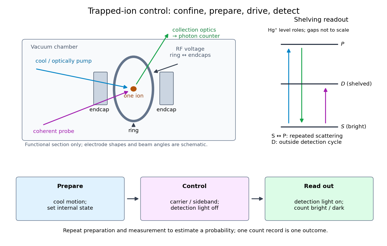
Trapped-ion quantum control prepares an ion's internal quantum state, couples it to quantized motion with laser pulses, and measures the result through state-dependent fluorescence. Its appeal is access to both a controllable two-level system and a quantum harmonic oscillator in one apparatus.
Confinement, preparation, control and readout solve different problems. The Paul trap's RF electric field confines the ion through its RF-averaged trapping potential; it still produces Paul trap micromotion. Doppler cooling and resolved sideband cooling reduce motional excitation. Optical pumping selects an internal quantum state. A coherent pulse then changes amplitudes, while electron shelving converts an internal population into a detectable stream of photons. A bright/dark count by itself does not reveal a quantum superposition's relative phase; an additional controlled rotation before detection can make that phase affect the measured population.

Semiconductor mass-action law Created 2026-10-18 Updated 2026-10-20
In thermal equilibrium, nondegenerate conduction electrons and valence electron holes share one chemical potential. Multiplying by cancels that chemical potential:This relation remains valid with semiconductor doping under the stated assumptions. Equality of the two individual densities, , additionally requires the intrinsic neutral case. Separate electron and hole quasi-Fermi levels in nonequilibrium need not obey this equilibrium product.
With one parabolic valley and two spin states at each band edge, the prefactor multiplying in the product is . Both populations must be nondegenerate; the Pauli reduction of the pinned-edge mass-action product quantifies a failure of the classical approximation.
For fixed band effective masses and band gap , the intrinsic carrier concentration obeys . ThusA base-ten plot against instead has slope after the prefactor correction. The intrinsic branch must be used, rather than the extrinsic plateau or dopant freeze-out branch. A changing gap or effective mass makes this an activation-energy estimate, and a small gap uncertainty can produce a much larger multiplicative uncertainty in a room-temperature minority density.
In a nondegenerate parabolic-band semiconductor with fixed density-of-states mass, , where . ThusA single measured value of does not determine its temperature dependence. A fixed-gap intrinsic model instead has , with the two effective density of states factors in . Identifying a crossover by gives an order-of-magnitude dopant-density estimate once that activation law is specified. At exact charge neutrality with , the total mobile-electron density is , so a crossover is not a sharp equality of every density definition.
Weighted interval scheduling 2026-10-18
Weighted interval scheduling assigns each job a reward and maximizes their sum over compatible jobs. Earliest finish can fail for this different objective function; dynamic programming can compare alternatives.[ref]
Lecture 1: Introduction. 6.046J Design and Analysis of Algorithms, Spring 2015; Printed pp. 4–5, Weighted Interval Scheduling and Dynamic Programming
For a separate two-job example, let have reward one and reward ten. Earliest finish accepts and rejects , earning one; the optimum accepts , earning ten. Replacing by preserves job count but loses reward. Thus the interval scheduling exchange argument proves the unit-value theorem only: its preserved quantity must match the intended objective function.
In this separate three-job example, labels denote new jobs:Their durations are five, five and two. Consider the rule "accept a shortest remaining job, discard all jobs conflicting with it, and repeat". It selects first. But overlaps on and on , so both are discarded. The rule returns one job, while the compatible subset contains two. The common endpoint five is allowed, and no feasible solution contains all three jobs, so two is the maximum.
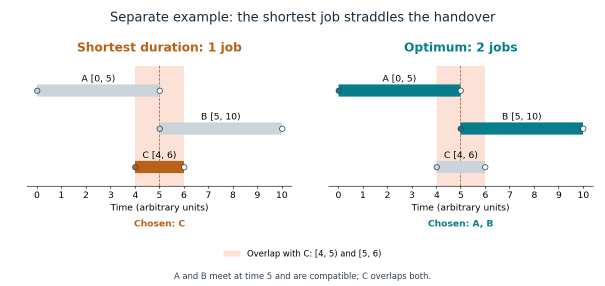
A two-unit job blocks two compatible five-unit jobs
. A separate three-job counterexample to choosing shortest duration. The left panel accepts only ; the right panel accepts and . Shaded bands mark the two positive-length overlaps with . Details.
Duration alone ignores where a job sits. Here the shortest job straddles the useful handover time. Earliest finish instead chooses , then , and attains two. A counterexample can refute a proposed greedy-choice property even when the rule succeeds on many other inputs.
For a well , choose normalized energy eigenstates , . The diagonal position matrix elements vanish by the parity operator. For ,To derive it, set and use . For unequal positive integer indices , the constant part of integrates to zero by orthogonality, whileTaking the difference for and yields the formula after setting . It vanishes for equal parity and gives for this phase convention.
For an infinite square well on , choose and , . The state has constant expectation value , butIndeed, the diagonal position matrix elements are , whereas the off-diagonal element isA different initial relative phase shifts the oscillation in time. The oscillation comes from quantum interference, while the constant mean energy follows from the fixed populations of the two energy eigenstates.
Boundary force in an infinite square well 2026-10-18
For a normalized sufficiently regular solution of the Schrödinger equation on with Dirichlet walls, the instantaneous outward forces on the walls have magnitudesA wall displacement changes the kinetic-energy quadratic form by the boundary term , giving the local force. Equivalently, direct integration by parts in the time derivative of the mean particle momentum givesThe force on the particle is the opposite of the net force on the walls. For a stationary energy eigenstate each magnitude equals . For the equal superposition of the first two box states, writing and gives and . Both time averages equal , the classical mean force on one wall at that energy, even though the quantum forces vary continuously in time.
Ground state at the top of a central rectangular barrier Created 2026-10-18 Updated 2026-10-20
Consider hard walls at , zero potential energy on and , and a central rectangular barrier whose height equals the ground state energy . The time-independent Schrödinger equation gives on the central interval. Reflection symmetry and the nodeless theorem for a one-dimensional ground state require an even, positive state about , hence a constant central segment. Wavefunction matching at a finite potential step makes the derivatives vanish at . The side segments are proportional to and . Their common plateau value is after wavefunction normalization, and . Equality of barrier height and energy is essential: a higher barrier gives positive curvature of a positive wavefunction in the middle, while a lower barrier gives negative curvature.
Mutual inductance 2026-10-18
For two fixed linear coils, mutual inductance relates magnetic flux linkage in one coil to electric current in the other: . The induced electromotive force is with consistent winding orientations. For reciprocal coils, , where are self-inductances and measures magnetic coupling. Its SI unit is the henry.
Inductance of a toroidal winding Created 2026-10-18 Updated 2026-11-05
For a slender winding around a toroid with turns, core area , mean magnetic path length and approximately constant magnetic permeability , Ampère's law gives . The linked magnetic flux is , so . This approximation neglects flux leakage and variation across the core and assumes operation below magnetic saturation. With a nonlinear magnetic core, an incremental inductance instead depends on differential permeability at the operating point.
A modern teaching experiment slows gravity-driven motion enough to resolve it with a photogate. PASCO scientific's Inclined Plane Dynamics Set, ME-6966, Instruction Manual 012-10874A describes “Acceleration Down an Incline” on printed pages 15–16. Its apparatus is a GOcar on a PAStrack with an adjustable incline support, a bracket-mounted photogate, a cart-mounted picket fence, and an interface with recording software. For the interface method, the fence's pattern is aligned to interrupt the beam. Recording starts before release from rest; the cart is caught at the bottom bumper. The procedure specifies three runs per angle, starting at and reducing by , with the release position fixed. The readout is velocity against time; its slope estimates acceleration. Mean accelerations are plotted against , testing the ideal slope . An added-mass comparison is also requested. These are protocol settings, not observed results.[ref]
The cart undergoes rolling without slipping at its wheels, whereas the worked block undergoes contact slip. Even ideal wheel moment of inertia changes the cart prediction. For total cart mass , wheel radii and axial moments of inertia , rigid wheels with fixed axles and no losses giveTo derive it, combine translational kinetic energy with wheel rotational kinetic energy , then equate their rate of change to the release of gravitational potential energy . This is the multiwheel counterpart of rolling acceleration with rotational inertia. Neglecting wheel moment of inertia yields ; treating a cart as a solid rolling cylinder would give a different correction.
Useful additional controls are repeated releases without a push, checking the fence alignment and spacing, and checking that the recorded velocity trace is straight over the fitted interval. A gently moving cart on a level track can expose losses or unintended tilt. These checks help distinguish an angle or timing error from neglected wheel moment of inertia, bearing friction, or drag force. The three-run spread measures repeatability but cannot by itself reveal a shared calibration error. The inspected protocol makes the gravity component measurable; it does not measure the sliding block's coefficient of kinetic friction.
Sliding acceleration on an inclined plane 2026-10-18
First test rest. With no other tangential forces, the required uphill static friction is . Its maximum is , where is the coefficient of static friction. ThusThe tangent function is increasing on this angle range, and its inverse tangent determines the last permitted resting angle . At equality, the ideal model still permits limiting rest; a larger angle excludes it. Below the threshold, setting would incorrectly impose the maximum static friction even when less is required. Static friction on an inclined plane and inclined-plane measurement of static friction develop this onset criterion further.
For a block already sliding downhill, uphill kinetic friction has magnitude , where is the coefficient of kinetic friction. Taking downhill as positive, Newton's second law becomesEvery term in the force balance scales with mass; division by removes it. Doubling mass doubles both gravitational weight and the contact forces, while leaving this acceleration unchanged if the coefficients remain unchanged. A mass-independent result is a prediction of these assumptions, rather than a universal property of every ramp.
For an original numerical model, stipulate , , and . The critical angle is . At , the normal force is ; rest requires of uphill static friction, below its bound. A resting block can stay there. If it is already sliding downhill, however, the kinetic friction is only , giving downhill acceleration . Specifying the initial state matters.
At , the downhill component of gravitational weight is , while and the static friction bound is only . Rest is impossible. During downhill sliding,Released from rest on a sufficiently long ramp, this ideal block covers its first in , reaching speed . As an independent energy calculation, the lost gravitational potential energy is and kinetic friction removes of mechanical energy. The remaining equals by the work-energy theorem.
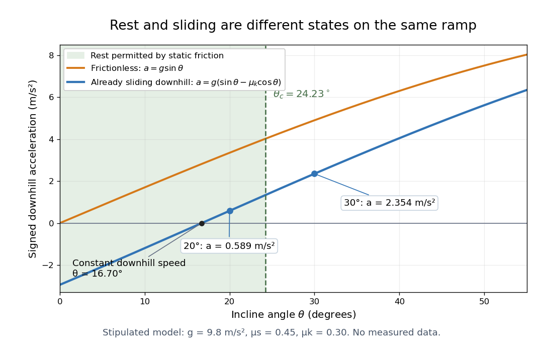

At , downhill sliding has zero acceleration and therefore constant velocity. Below that angle, a downhill-moving block slows; when it stops, test the static friction bound again. For uphill sliding, kinetic friction points downhill, so the signed downhill acceleration instead is . The sign follows contact slip, and the downhill formula cannot be used unchanged after a reversal.
Gravity components on an inclined plane 2026-10-18
Choose a unit vector pointing downhill and a perpendicular unit vector pointing outward from the inclined plane. The gravitational weight points vertically downward. Its scalar projections onto these directions giveThe angle between the downward vertical and the inward normal is : the inward component uses cosine, and the downhill component uses sine. These are two components of one force. They replace its vertical arrow in a component calculation; adding them to that same arrow would count gravitational weight twice.
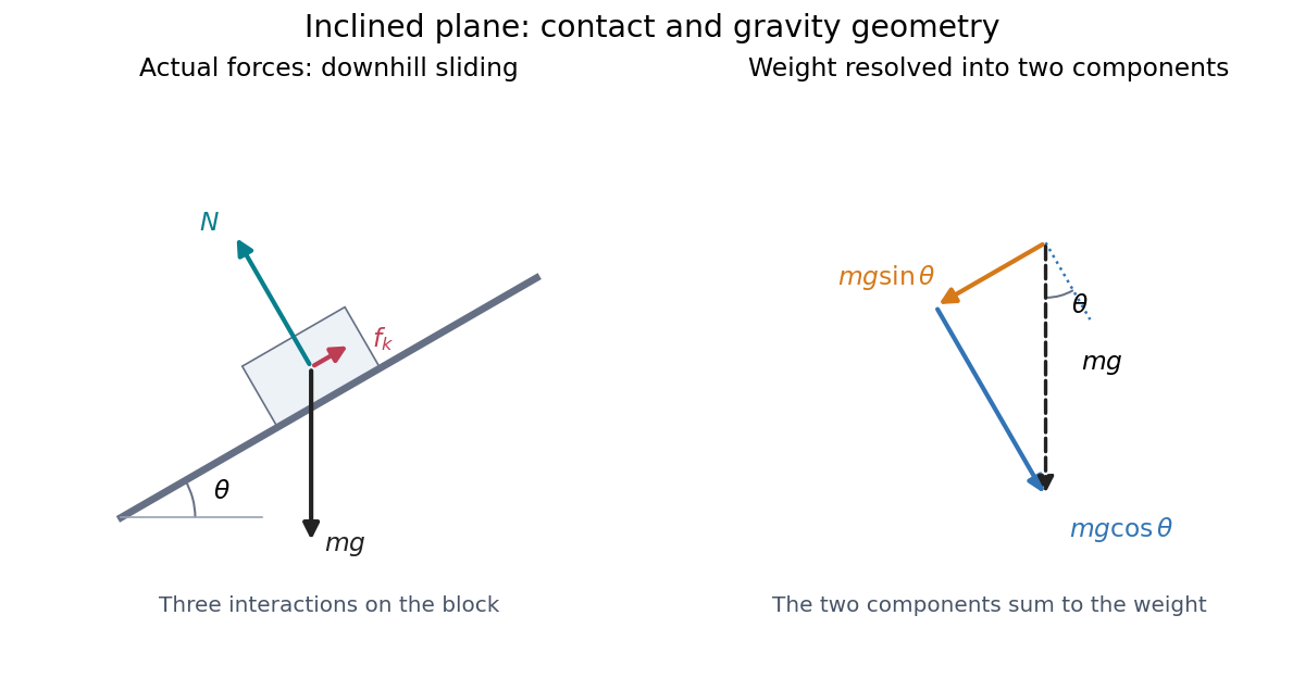

Continued contact with a stationary straight inclined plane gives zero perpendicular acceleration. The perpendicular component of Newton's second law therefore givesThis is why the normal force generally differs from : it balances the inward component, rather than the whole gravitational weight. An extra lifting force, a curved surface, or motion of the support would require a new perpendicular balance.[ref]
6.2 Friction. University Physics Volume 1 by William Moebs and others; “Friction and the Inclined Plane”, Example 6.11 strategy and Figure 6.14; perpendicular balance and
The same geometry explains the ramp's usefulness. A frictionless block pulled uphill at constant velocity needs a parallel force . Travelling a distance raises it through height , so the pulling work is , its gain in gravitational potential energy. The smaller force costs a larger displacement; the work-energy theorem keeps the accounting consistent.
List of immunologists 2026-10-18
Antibody hinge region 2026-10-18
The antibody hinge region is a flexible IgG immunoglobulin heavy chain segment between and containing inter-heavy-chain disulfide bonds.[ref]
The structure of a typical antibody molecule. Immunobiology: The Immune System in Health and Disease, 5th edition by Charles A. Janeway, Jr. and others; §3-3 and Figure 3.3: hinge and cleavage on the amino-terminal side of its inter-heavy-chain disulfides
IgG chain reduction experiment 2026-10-18
Gerald M. Edelman reduced IgG disulfide bonds and used dissociating chemical solutions, including urea. Ultracentrifugal analysis showed a decrease in molar mass, supporting a multichain protein. In the comparison reproduced in his lecture, starch gel electrophoresis in urea separated serum IgG and a urinary protein from the same patient, alongside their reduced and alkylation-treated preparations. The untreated samples provided the treatment comparison; the urinary material provided a chain-identity comparison. The treated serum sample revealed heavy- and light-chain bands. Two-dimensional peptide mapping compared the urinary protein with the isolated immunoglobulin light chain. Together these readouts supported a shared chain identity.[ref]
Antibody Structure and Molecular Immunology by Gerald M. Edelman. Gerald M. Edelman, Antibody Structure and Molecular Immunology, Nobel Lecture dated 12 December 1972, printed pp. 33–34 and Figure 2a–b: dissociation, four comparison lanes and peptide maps
The controls address distinct alternatives. Treatment-dependent separation supports chains joined in the starting protein; a matching gel electrophoresis position alone would not uniquely identify a chain. Agreement of peptide mapping adds an independent chemical comparison. Neither readout gives atomic coordinates, and this patient's preparation does not establish a common protein primary structure for all antibodies.
Reduction targets protein disulfide bonds, while protein denaturation weakens the folded assembly. Neither operation is the proteolysis that cuts peptide bonds. This explains why chain separation and Papain digestion of IgG give different inventories: four intact chain backbones in the first case, three assembled fragments in the second.
Work by Immanuel Estermann 2026-10-18
There are unlisted articles, also show them or only show them.