
For a finite Galois extension of number fields and a finite-dimensional complex group representation of its Galois group, the finite part of its Artin L-function is the Euler productHere is the inertia group, and a Frobenius automorphism lift acts on its invariant subspace. Different lifts induce the same operator there. At an unramified prime the invariant subspace is all of ; at a ramified prime this restriction removes the part on which inertia acts nontrivially.
The trivial representation gives the Dedekind zeta function of . Direct sums of representations give products of Artin L-functions, because determinants multiply on direct sums. Taking the logarithm of each local factor produces traces of powers of Frobenius, connecting representation-theoretic characters with prime-counting sums. Archimedean factors are added separately when forming a completed L-function.
For a cyclic extension of number fields, an element of the base field is a global field norm exactly when it is a norm at every finite and infinite completion. The splitting criterion for a cyclic algebra encodes the norm obstruction as a Brauer group class. The Albert-Brauer-Hasse-Noether theorem makes a class that splits at every completion split globally, giving the result. Cyclicity is essential; arbitrary noncyclic extensions can have additional local-global norm obstructions.
Citrate denotes an ion derived from citric acid. The commonly specified form has electric charge equal to that of three electrons and chemical formula ; it results from removing three hydrogen ions from citric acid. Forms with additional hydrogen ions attached through protonation also occur. [ref]
https://www.ebi.ac.uk/chebi/CHEBI:16947. ChEBI, citrate(3−)
In an inviscid barotropic fluid subject to conservative body force, the circulation of a material loop is constant. For constant density, parameterize that loop by with . Differentiating gives an integral of plus . The latter vanishes on a closed loop, and the Euler equations make the former the integral of a gradient, also zero. For a barotropic density, is still a gradient of specific enthalpy. Constant circulation is consistent with changing local vorticity when a vortex tube changes its cross-sectional area.
In a spherically symmetric gravitational potential , a circular orbit has , specific orbital energy and specific angular momentum , with . Differentiating gives . Changes in orbital orientation have , so . For a particle of variable mass and total angular momentum , this implies . Moreover , which is positive when the orbital angular velocity decreases outward.
For a fixed spherical gravitating source, place a test particle at with initial velocity , where is outside the source. Its exact circular orbit isDifferentiating twice gives , precisely the Newtonian gravitational field at each point of that circle. There is no outward physical force to cancel gravity in this inertial frame. Gravity supplies the inward centripetal acceleration that continually changes the velocity's direction.
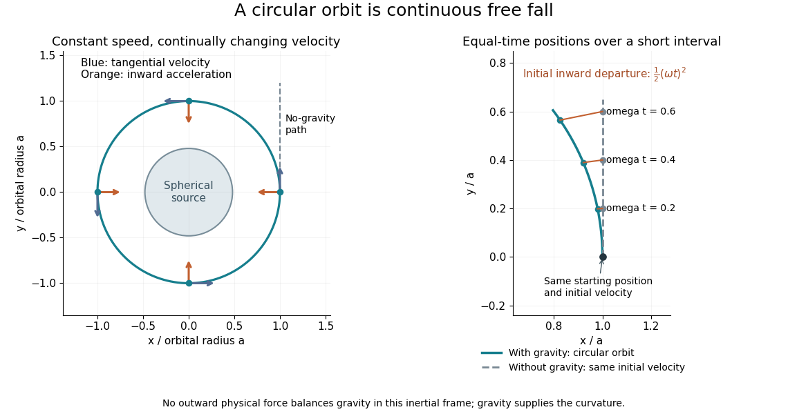
A circular free-fall orbit, inward acceleration, and the straight path the same initial velocity would produce without gravity
. Details. Over a short interval, the displacement from the straight tangent path begins inward with magnitude . The curvature of the orbit matters at the same order: the particle moves sideways while continually falling away from its instantaneous tangent. The full circular solution remains at radius rather than striking the source.
Its speed is , its oscillation period is , and its specific orbital energy is . Removing gravity while keeping the initial velocity would give the straight path , rather than a stationary particle. This contrast explains why orbital weightlessness is compatible with a substantial gravitational force: a freely coasting spacecraft and its contents fall together. [ref]
https://www.nasa.gov/centers-and-facilities/glenn/what-is-microgravity/. NASA Glenn: orbit as continuous free fall and the origin of weightlessness
Consider the discrete linear system withThis is a finite periodic analogue of the Poisson equation, using the negative second finite difference with unit grid spacing. It is also a Graph Laplacian equation on a cycle graph; no continuum approximation is being claimed here.
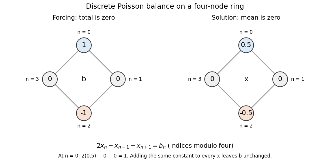


Summing the four equations gives zero on the left, since each value occurs twice positively and twice negatively. A necessary condition is therefore . The Fourier diagonalization of a circulant matrix shows that this is also sufficient: the only zero eigenvalue of is the constant mode , and .
For the displayed forcing, the discrete Fourier transform givesDivide only at the three nonzero eigenvalues, and choose to impose zero arithmetic mean:Direct substitution gives . All other vectors satisfying the linear system are , because the kernel is the space of constant vectors. Thus balanced forcing determines the differences between values, while a reference level is an extra choice. This small model explains why a periodic Poisson equation needs both a compatibility condition and a normalization.
Use the negative-exponential forward discrete Fourier transform and the -normalized inverse discrete Fourier transform:For the circulant matrix with first column , the discrete Fourier mode is an eigenvector with eigenvalueIndeed, substitution into circular convolution givesThe columns of are , so the diagonalization of a matrix takes the formThe roots of unity give orthogonality of these eigenvectors; dividing each by makes the basis orthonormal. Consequently, every complex circulant matrix is a normal matrix, including ones that are not Hermitian matrices.
The sign convention matters. For , the circulant matrix isChanging the direction of the shift or the sign in the discrete Fourier transform changes which complex eigenvalue goes with which discrete Fourier mode. A real symmetric example alone would conceal that distinction.
For a linear system , put and . The equation becomes independent scalar equationsIf every is nonzero, divide to find the unique vector and apply the inverse discrete Fourier transform. If some , a vector satisfying the linear system exists exactly when at every such index; the corresponding remain free. This is a concrete version of the Fredholm alternative in a finite-dimensional setting.
With an appropriate Fast Fourier transform, multiplication or a compatible solve takes arithmetic operations, instead of forming a dense matrix and applying general Gaussian elimination. The gain comes from the periodic structure; an arbitrary matrix does not have this shared basis of discrete Fourier modes.[ref]
A perfect elimination ordering of a finite simple graph is a permutation of its vertices such that each set of later graph neighboursis a clique. Thus is a simplicial vertex in the remaining induced subgraph . Empty and one-vertex sets satisfy the clique condition automatically. The order here is the order of deletion: goes first.
The characterization is powerful: a finite simple graph is a chordal graph if and only if it has a perfect elimination ordering. For one proof outline, the earliest vertex of an induced cycle of length at least four would have two later graph neighbours on that graph cycle that are not adjacent, contradicting the clique condition. Conversely, every nonempty chordal graph has a simplicial vertex, and every induced subgraph of a chordal graph is a chordal graph; repeatedly deleting such a vertex supplies the ordering.[ref]
In the square-plus-diagonal chordal graph above, is a perfect elimination ordering, with later graph neighbourhoods , , , and . Starting instead with fails: its graph neighbours do not form a clique, because is absent. Thus even a chordal graph can have a poor elimination ordering.
For a larger example, join three triangles along shared edges, usingThe exact graph neighbourhoods are , , , , and . The ordering has later graph neighbourhoods , , , , and , all cliques; this certifies that the graph is a chordal graph without enumerating its graph cycles. Its maximal cliques , , form a junction tree in that order, with intersections and .
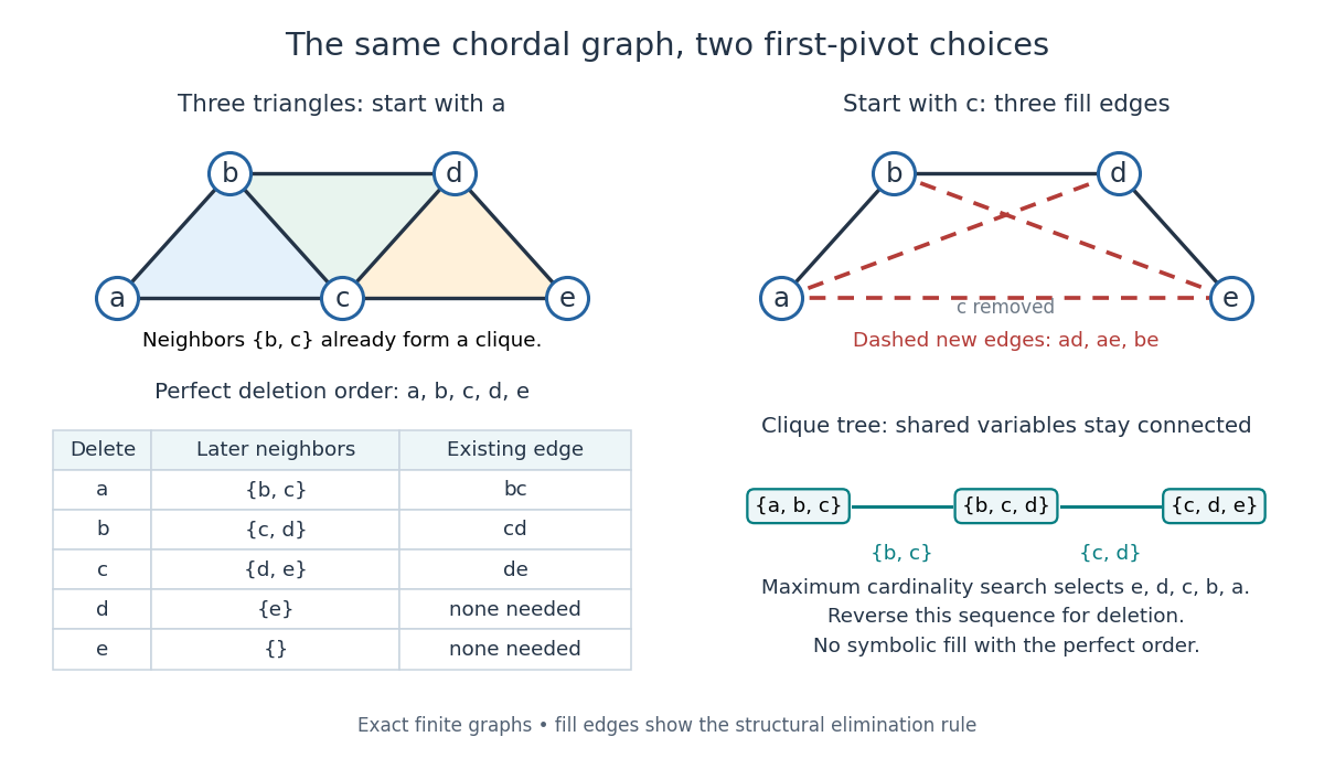
A perfect elimination ordering removes three overlapping triangles without fill-in; choosing the central vertex first adds three edges
. Details. 
To find an ordering, maximum cardinality search starts with all scores zero, repeatedly selects an unselected vertex of largest score, and increases each unselected graph neighbour's score by one. Reverse the selection order to obtain a candidate perfect elimination ordering. For the three-triangle graph, one valid selection sequence is , with scores at selection ; reversing it gives the displayed deletion order. On a chordal graph every tie choice works. On an arbitrary graph, test the resulting later graph neighbourhoods for the clique condition to recognize chordal graphs. Suitable adjacency lists, score buckets and a linear-time verification method give recognition.[ref]
The deletion rule also explains sparse Gaussian elimination. For a symmetric positive-definite matrix whose matrix graph is , eliminating pivot applies the Schur complement updateOnly pairs of remaining graph neighbours of can acquire new off-diagonal entries. A perfect elimination ordering already has all those edges, so Cholesky decomposition creates no symbolic fill-in. Positive definiteness ensures nonzero pivots in exact arithmetic. Special numerical cancellation can suppress predicted entries, and floating-point rounding affects their values.[ref]
Chordal Graphs and Semidefinite Optimization by Lieven Vandenberghe and others. §9.1; equation 9.2; Theorem 9.1
In the three-triangle graph, deleting first instead connects every pair in and adds exactly . The graph was already a chordal graph; the extra fill-in comes from the ordering.One further reward is optimal graph coloring. Process a perfect elimination ordering backwards and give each vertex the smallest positive color absent from its already colored graph neighbours. Those graph neighbours form a clique, so this greedy algorithm uses at most the clique number colors; any clique of that size requires at least that many. In the three-triangle graph, coloring gives colors , so both the chromatic number and the clique number are three. Every maximal clique also occurs among : take its earliest vertex and use maximality. The same ordering therefore supports graph coloring, maximal clique extraction and sparse computation.
Historically, Donald J. Rose, Robert E. Tarjan and George S. Lueker's 1976 paper connected graph elimination to symmetric sparse matrices and gave a search-based algorithm for finding a perfect elimination ordering when one exists. Its abstract distinguishes a minimal elimination ordering from a minimum one: removing avoidable fill-in does not by itself minimize the total number of added edges.[ref]
Triangulation adds fill edges to an undirected graph to make it a chordal graph. Given an elimination ordering, join all remaining neighbors of each removed vertex. The completed graph has that perfect elimination ordering. Fill edges can enlarge the cliques used for exact probabilistic graphical model inference, without changing the original probability factors; they do not assert new biological relationships.
The chemotaxis FRET assay uses Förster resonance energy transfer between fluorescent tags on CheY and CheZ to report their association. Interpreting this emission ratio as CheA activity requires the coupling between CheY phosphorylation and CheZ binding described in the experimental sources above.
Chemotaxis feedback proteins alter the internal signalling state of a chemotactic cell in response to pathway activity. In the canonical Escherichia coli system, CheR adds receptor methyl groups and CheB removes them, with CheB activity coupled to phosphorylation. Their opposing actions help restore receptor-pathway output after a persistent stimulus. This changes response sensitivity while allowing continued detection of subsequent changes in attractant concentration. [ref]
Robustness in simple biochemical networks by Naama Barkai and Stanislas Leibler. 1997, methylation-demethylation feedback architecture
The Tar receptor is an Escherichia coli chemoreceptor that detects attractant signals including aspartate. Receptor arrays regulate the kinase pathway controlling motor behaviour, while receptor methylation helps adjust sensitivity after sustained stimulation. Ligand recognition, kinase output and adaptation are different stages, so a binding measurement alone does not establish the swimming response. [ref]
UniProtKB by the UniProt Consortium. P07017, Function, Catalytic activity and Subunit structure
Receptor methylation is covalent addition of methyl groups to a receptor. In bacterial chemotaxis, reversible modification of chemoreceptor residues changes signalling sensitivity and contributes to signaling adaptation. Methylation and demethylation act on the internal response state while external ligand concentration can remain changed. This provides a biochemical memory of recent stimulation rather than removing the stimulus from the environment. [ref]
Robustness in simple biochemical networks by Naama Barkai and Stanislas Leibler. 1997, receptor modification and robust adaptation model
Shunting inhibition is suppression of another input's effect through increased synaptic conductance: opening additional ion channels lowers effective electrical resistance, reducing the voltage response to a given added electric current. When the added reversal potential equals the resting membrane potential, there can be no voltage change at rest and still be inhibition of a simultaneous input. See 1.4 Limitations of the Leaky Integrate-and-Fire Model.
Use the passive synaptic potential model below with leak , and capacitance . A sustained inward test electric current of alone gives a steady voltage increase of , so . Effective electrical resistance is and the time constant is .
Now hold a shunting conductance open with . With no test electric current, rest stays at . With the same test electric current, total conductance becomes , so the steady voltage increase is only : . Effective electrical resistance is and the time constant is . A faster response can therefore be smaller. At the original rest the shunting electric current is zero; at it is , opposing the voltage excursion.
The factor of three reduction applies to this constant-electric current, constant-conductance example. A finite pulse, conductance-driven input or spatially extended dendrite need not have the same reduction. The interesting feature is conditional action: the shunt can leave a quiet neuron's voltage unchanged yet reshape its response when another input arrives. A model that represents all inhibition as a fixed outward electric current misses this behavior.
A synaptic vesicle is a small membrane-bounded compartment in a presynaptic terminal that stores neurotransmitter for release. Fusion with the cell membrane exposes its contents to the synaptic cleft; the packet supplied by one synaptic vesicle is a quantum of release. Quantal neurotransmitter release refers to these discrete packets, rather than the release of one molecule at a time. The postsynaptic response to a packet can vary with its contents, receptors and recording conditions. See Purves and colleagues: vesicles as the source of transmitter quanta.
The useful cycle is filling, preparation for fusion, calcium-triggered exocytosis, and recovery of membrane and proteins through endocytosis for reuse. Different recovery routes occur; recycling need not preserve a particular synaptic vesicle as an identifiable container throughout. Limited availability of prepared synaptic vesicles can reduce release during repeated stimulation, while changes in synaptic release probability can also change successive responses. See Basic Neurochemistry: secretion machinery and vesicle reuse and 3.1 Synapses.
For an illustrative calculation, assume four release sites, each with one prepared synaptic vesicle, each releasing with synaptic release probability during one presynaptic action potential. Assume independent Bernoulli trials and at most one release per site. The released packet count has a binomial distribution:The probability of no release is ; at least one release has probability . An expected value of one packet does not mean that every action potential releases one packet. If each packet contributes a stipulated conductance increment and increments add, the expected value of that increment is , with zero increment on about of trials. These assumptions are a teaching model: shared calcium fluctuations, unequal sites, depletion and nonlinear receptor responses can invalidate them.
The synaptic cleft is the extracellular gap between the sending and receiving cell membranes of a chemical synapse. Released neurotransmitter crosses this gap to reach a receptor. [ref]
Neurotransmitter clearance removes released neurotransmitter from the region where it can activate receptors, through diffusion, cellular uptake or enzyme-mediated breakdown. Its routes and rates help delimit a chemical synapse's response in space and time; see the mechanisms and source under chemical synapse.
The molar electrochemical potential combines the molar chemical potential with the electrical contribution , where is the signed charge number of an ion, is the Faraday constant and is electric potential. Both terms have units . In the particle convention the corresponding expression is , with elementary charge ; multiplying it by the Avogadro constant gives the molar form. Transfer between locations at the same temperature and pressure is driven by differences in electrochemical potential. The membrane transport examples use it to distinguish neutral solute transfer from ion transfer.
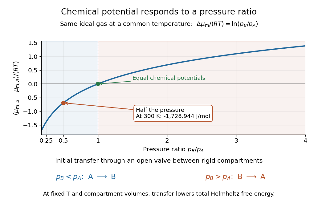
For a pure ideal gas at temperature and pressure ,where is the molar gas constant and specifies the reference pressure of the standard state. The ratio inside the natural logarithm is dimensionless. The chemical potential difference therefore depends on a ratio of pressures, not an absolute difference. See MIT 5.60, Lecture 14, page 4.
For a chemical species in an ideal gas mixture, replace by its partial pressure. More generally write using its thermodynamic activity and a consistent standard state. For an ideal dilute chemical solution, with reference concentration ; the thermodynamic activity section describes departures from this idealization.
As a computed comparison, take identical chemical species at , with and . Stipulate . ThenHalving the pressure gives the same decrement whether starting from or , provided the ideal gas approximation remains valid. This comparison uses different pressures; it is not the common-pressure reservoir setup of chemical potential equality for particle exchange. The fixed-volume example in chemical potential and Helmholtz free energy supplies an exchange experiment with unequal initial pressures.

There are unlisted articles, also show them or only show them.