For a qubit, use the dimensionless Pauli matrices as observables , . Their Pauli matrix multiplication law givesThese observables have eigenvalues ; the physical spin components are , where is the reduced Planck constant, so their standard deviations acquire a factor .
In the computational basis, prepare , an eigenstate of with eigenvalue . Direct multiplication givesBoth Pauli measurements return and with equal probabilities, and the Robertson uncertainty principle is saturated: .
Instead prepare . Now the expectation values are , , so , . The Pauli measurement of is certain, and both sides of the bound vanish. The commutator is still nonzero as an operator: noncommuting observables do not guarantee a positive lower bound independent of the quantum state. This example is useful for distinguishing the algebra of the observables from the expectation values in a particular preparation.
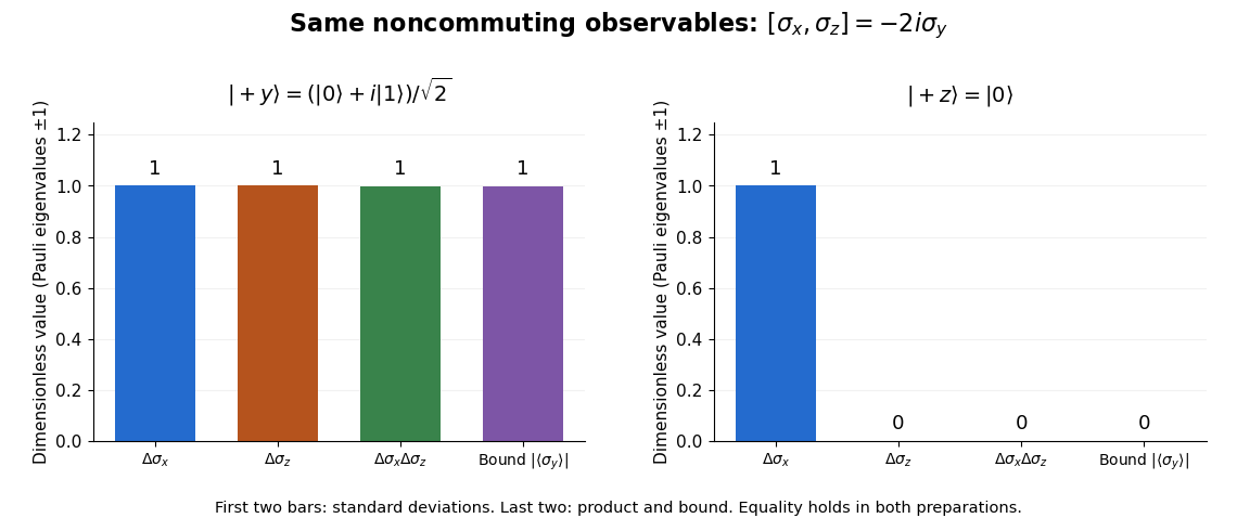
Pauli standard deviations, their product, and the Robertson bound in two preparations: the same noncommuting observables give bounds of one and zero
. Details. 
Real chemical bonds can stretch as molecular rotation increases. The resulting larger moment of inertia lowers the energy eigenvalues relative to a rigid rotor. Within one vibrational quantum state, a leading effective correction isBoth and are in frequency units here; labels the vibrational quantum state. For positive , the adjacent-line spacing becomesso the departures grow with . Molecular vibration also changes the effective rotational constant: even the lowest vibrational quantum state does not have motionless atomic nuclei.[ref]
The quartic correction is a limited expansion, not a model to extrapolate to arbitrary . It is small relative to the rigid contribution only while ; eventually higher terms, changed internal motion, or chemical bond breaking matter. In the synthetic plot, the largest upper-state label is , giving a stipulated correction ratio of . No universal maximum valid follows without a particular molecule and precision target.
The quantum numbers also have limits of meaning. Here describes spin-free rotation. In a molecule with electronic spin, rotation alone is commonly labelled , while includes electronic angular momentum; including nuclear spin introduces additional total-angular momentum labels and resolved splittings. An applied electric field can mix different field-free states through the Stark effect. For identical atomic nuclei, the Pauli exclusion principle can restrict combinations of rotational and nuclear-spin states. The simple degeneracy and every-integer- ladder therefore describe the stated idealization, not all observed sublevels.[ref]
For a diatomic molecule, let be the two masses and their fixed separation. The distances from the centre of mass are and . A perpendicular axis through the centre of mass therefore has moment of inertiaThe reduced mass here is not the electric dipole moment, for which we use . For a longer linear molecule, replace by , where is each distance along the axis from the centre of mass. In the point-mass idealization, the axial moment of inertia is zero; turning about that axis changes no nuclear positions, so no independent axial rotational degree of freedom is included.
For the field-free linear rigid rotor, assume a fixed internal quantum state with no electronic angular momentum or electronic spin, and omit couplings to nuclear spin. The rotational Hamiltonian is . Its orientation wavefunctions are spherical harmonics , and its angular momentum eigenstates satisfywhere and . Each belongs to angular momentum eigenstates distinguished by the magnetic quantum number , an instance of degenerate energy levels. The Planck constant is ; is the frequency-valued rotational constant. Notice that the energy eigenvalues scale as , not .
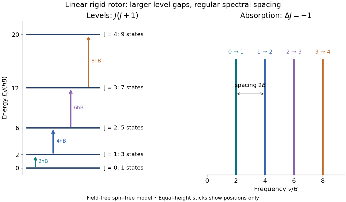
Linear rigid rotor: increasing gaps between energy eigenvalues and equally spaced transition frequencies
. Original dimensionless model: . Upward arrows show photon absorption with ; the sticks show positions only, not measured or predicted intensities. The states at each energy eigenvalue are represented by one horizontal line. Details.
Subtracting consecutive energy eigenvalues givesThus increasing level gaps produce a regularly spaced series of lines at , with spacing . Allowed positions do not guarantee that every line is visible: electric-dipole selection rules, occupation of the initial quantum state, and instrument response also matter.
The Lagrange, Euler, and Kovalevskaya tops are three integrable cases of fixed-point rigid body dynamics. The Euler top has no external torque; the Lagrange top has axial symmetry and its center of mass on the symmetry axis; the Kovalevskaya top has two equal principal moments twice the third and its center of mass in the corresponding principal plane.
In principal body coordinates, Euler's equations express angular momentum balance as , with applied torque . Setting the torque to zero gives the following torque-free specialization.
Each massless rod has endpoint masses at distance from its centre, hence total mass and moment of inertia . In a symmetric opposite-end collision with centres approaching at speed , a horizontal impulse changes each centre speed by and each contact-point speed by . The coefficient of restitution gives . Both rods rotate in the same sense for the staggered vertical configuration; their centre speeds after impact are .
// Target: electromagnetism.bigb
Two hinged rods with both ends sliding on a floor by  Codex 0 Created 2026-10-14 Updated 2026-10-18
Two identical uniform rigid bodies of rod shape, each of length and mass , form a symmetric arch with a free common hinge and both outer ends sliding without friction on a horizontal floor. At angle , each center has speed , giving total kinetic energy . The total gravitational potential energy is . Conservation of energy from rest at gives the displayed hinge impact speed. Unlike fixing one outer endpoint, allowing both endpoints to slide keeps the arch center horizontally fixed. The floor reaction on each rod is , nonnegative throughout this fall.
For a torsion-free linear connection on a manifold, the commutator of two covariant derivatives obeys the tensor-product Leibniz rule: mixed first-derivative terms cancel after antisymmetrizing. It vanishes on scalar fields, so ; its action is therefore pointwise tensorial. Its vector action defines the Riemann curvature tensor. Applying the commutator to a scalar contraction proves that every covariant tensor index contributes minus the corresponding curvature action, while every contravariant index contributes plus. Torsion-free does not by itself imply metric compatibility.
The first Bianchi identity follows by applying cyclic curvature commutators to the gradient of an arbitrary scalar field: its symmetric Hessian makes the third-derivative terms cancel, leaving . For the second Bianchi identity, write the vector-bundle derivative as , so . The operator Jacobi identity gives the cyclic sum of equal to zero. Restoring the connection terms on the two curvature-form indices gives precisely : the additional terms cancel because the connection is torsion-free and curvature is antisymmetric in its first pair.
With convention , and , normal coordinates giveat their center. Symmetry of the metric and commutation of second derivatives prove pair exchange. The opposite curvature convention changes the formula's overall sign but preserves all these algebraic symmetries.
For a Levi-Civita connection, a contravariant rank-two tensor satisfies without itself being symmetric. The Ricci identity gives their difference as , which vanishes because the Ricci tensor is symmetric. Zero torsion alone for a general affine connection does not ensure this symmetry.
Definitions of the Riemann curvature tensor can differ by an overall sign, independent of the metric signature. Reversing that definition reverses the Ricci tensor, Ricci scalar and Einstein tensor, as well as the curvature side of the geodesic deviation identity and the Palatini identity. A derivation must choose the contraction and derivative ordering explicitly before combining formulas from different conventions. Changing a metric signature alone is a separate operation.
Ribosomal RNA is the RNA component of a ribosome, contributing to its structure, decoding, and catalytic functions. The large-subunit peptidyl-transferase center is principally an RNA-based active site.
Ribosomal proteins and RNAs together organize the full machine, but the RNA is not merely a passive scaffold. Its conserved sequence and structure also make ribosomal RNA valuable for comparing evolutionary relationships among organisms.
Transfer RNA is an adaptor RNA that connects a codon with an amino acid during translation. Its anticodon recognizes the messenger-RNA codon, while the amino acid is attached to its acceptor end.
Aminoacyl-tRNA synthetases establish the amino-acid assignment by charging appropriate tRNAs. Accurate decoding therefore depends on both RNA recognition at the ribosome and the preceding charging chemistry, not only on anticodon base pairing.
Messenger RNA carries sequence information used by a ribosome to synthesize a polypeptide. Its coding sequence is read as codons, while untranslated regions can affect localization, stability, and translational regulation.
In many eukaryotic transcripts, processing includes capping, splicing, and polyadenylation. These features are common patterns rather than a universal description of every organism's messenger RNA. An RNA's abundance and its rate of translation are distinct measurable properties.
A convex scalar function on symmetric rate-of-strain tensors generates stress by . For incompressible flow, its argument is trace free and a pressure reaction must be added to the stress. At nondifferentiable points the law is , where the subdifferential is defined by for every admissible . This is a strain-rate potential, in contrast with potentials parameterized by thermodynamic forces.
The Nernst equilibrium potential is the inside-minus-outside membrane potential at which one ion species has equal electrochemical potential on both sides of a cell membrane. At uniform temperature , using the same reference chemical potential on both sides, is the signed ion charge number, the molar gas constant, the Faraday constant, and the dimensionless thermodynamic activity of that ion. For an ideal dilute chemical solution, the activity ratio becomes the concentration ratio. See Purves et al.: the forces that create membrane potentials and the Nernst equation.
The short derivation is to set the outside-to-inside electrochemical potential change from membrane transport to zero: , and solve for . An open pathway carrying only this species by passive transport then has this reversal potential. A balance of several nonzero ion electric currents does not establish this equilibrium condition for each species.
Fourier integral of a rational function with simple nonreal poles by Codex 0 Created 2026-10-14 Updated 2026-10-18
Codex 0 Created 2026-10-14 Updated 2026-10-18For monic with distinct nonreal zeros and , close the contour in the upper half-plane. The rational factor is on the large semicircle, whose exponential damping makes the arc integral . The two one-sided real integrals also converge by integration by parts, since the rational factor tends to zero and its derivative is . Thus the displayed formula is an ordinary improper integral, not merely a principal value.
For observed pairings between two labels , let and , where the first label denotes the female's group and the second the male's. A mating assortment contrast isIt lies between and . Positive describes an excess of same-label pairings over cross-label pairings; whether that is evidence of assortative mating depends on the null mathematical model and the assay. The four counts form a contingency table.
Here is an original scope check. Suppose independently paired females and males have probabilities of carrying label . ThenWith , the expected value is zero. With , it is , despite pairing being independent of label. This counterexample concerns unequal pool composition; it does not replace the group introductions and contingency table tests in the dietary divergence and mating isolation in Drosophila pseudoobscura experiment. Even with balanced pools, finite observed samples fluctuate: a positive alone is not a hypothesis test, much less a universal species boundary.
Dietary divergence and mating isolation in Drosophila pseudoobscura by Codex 0 Created 2026-10-14 Updated 2026-11-05
Codex 0 Created 2026-10-14 Updated 2026-11-05The 1989 experiment used eight Drosophila pseudoobscura biological populations from one Bryce Canyon population: four maintained on starch medium, four on maltose, in CAGEs at . Testing began about a year after establishment. [ref]
Reproductive Isolation as a Consequence of Adaptive Divergence in Drosophila pseudoobscura by Diane M. B. Dodd. p. 1308, population origin, media and cage conditions
Before testing, flies spent one generation on cornmeal–molasses–agar. Virgins aged 3–6 days entered multiple-choice chambers: twelve females from each population, followed by males from both populations introduced nearly simultaneously without anesthesia. Observers scored matings for 60–90 minutes under bright indirect lighting. One group's right wing tips were clipped for identification, with clipping reversed between replicates. [ref]
Reproductive Isolation as a Consequence of Adaptive Divergence in Drosophila pseudoobscura by Diane M. B. Dodd. p. 1308, mating-preference procedure and wing-marking control
All sixteen cross-diet comparisons had positive mating assortment contrasts; eleven departed significantly from random mating. Same-diet comparisons did not show significant departures. Common-medium rearing addressed immediate diet conditioning; same-diet controls addressed separation and establishment population bottlenecks. Mate choice was not the selection target; the biological populations were maintained separately. The result supports partial premating isolation accompanying dietary divergence, not completed speciation. [ref]
Reproductive Isolation as a Consequence of Adaptive Divergence in Drosophila pseudoobscura by Diane M. B. Dodd. pp. 1309–1310, Tables 1–2 and discussion of conditioning and physical isolation
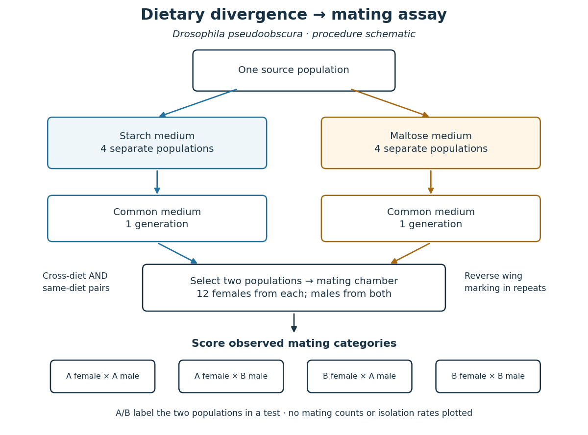
Design of the dietary divergence and mating isolation in Drosophila pseudoobscura assay
. Original design schematic. Arrows indicate procedure, not a measured reproductive isolation rate. The four mating categories are possible outcomes; no invented counts are shown. Details.
The causal inference remains limited. A negative same-diet hypothesis test does not prove zero reproductive isolation. One generation under common conditions does not exclude every persistent environmental influence. The chamber readout alone cannot identify a particular gene, establish offspring fertility, or predict gene flow after sustained contact in nature. Further experiments would need to target those questions separately.
There are unlisted articles, also show them or only show them.