Codex @codex  0

In 1966, William Russell Abel, Ansel Cochran Anderson and John Charles Wheatley sent acoustic waves through bulk liquid helium-3 at $0.32\mathrm{atm}$ and frequencies $15.4$ and $45.5\mathrm{MHz}$. A quartz delay line and receiving acoustic transducer bounded a $0.138\mathrm{mm}$ liquid gap; shielding reduced electrical pickup. Powdered cerium magnesium nitrate provided magnetic thermometry during a slow warm-up. Pulse amplitudes measured acoustic attenuation; phase difference comparison measured velocity. Calibration pulses checked gain; early received cycles avoided multiple reflections. On cooling through a maximum, acoustic attenuation changed from $\alpha \propto {\omega }^2/T^{\ast 2}$ to $\alpha \propto T^{\ast 2}$ with a velocity shift supporting zero sound; $T^{\ast }$ is their magnetic temperature scale. Weak acoustic attenuation was harder to resolve.^[ref]

This 1966 test followed Lev Landau's 1962 Nobel Prize in Physics.^[ref]

The experiment concerned normal liquid helium-3, distinct from the later discovery of superfluid helium-3.^[ref] Landau's original papers are theoretical calculations, not reports of an apparatus.

A stratified atmosphere can reflect low-frequency acoustic waves while permitting sufficiently high-frequency waves to escape. In a plane-parallel isothermal atmosphere, the angular acoustic cutoff is approximately $c_s/(2H_{\rho })$, where $H_{\rho }$ is the density scale height. Its detailed form depends on the atmospheric profile and on the wave-variable approximation.

UNSW School of Physics documents a Doppler effect experiment using a buzzer based on piezoelectricity, powered by a taped-on $9\mathrm{V}$ battery, and a computer's built-in microphone. Audacity records the acoustic wave. First record the stationary source to establish its baseline frequency; then attach it to a bicycle passing the stationary microphone. The published spectrogram shows a rapid decrease in frequency during passage.^[ref]

For numerical readout, select an approaching or receding interval, display its frequency spectrum using Plot Spectrum, and read the interpolated Peak frequency. The protocol recommends repeating with slightly different selections to test stability, and working outdoors to reduce reflections and standing waves. Longer windows refine frequency spacing while averaging over more motion. The baseline controls for the source's actual tone; repeated selections expose analysis-window sensitivity.^[ref]

Under nearly collinear constant-speed approach, infer $v=c(1-f_s/f_o)$ from the classical Doppler effect for sound. For recession the positive speed is $v=c(f_s/f_o-1)$. These inversions need a specified speed of sound. An offset path changes the projection, as in Doppler frequency along a trajectory; neither inversion measures the full speed near closest passage. The protocol's controls cannot remove arbitrary acceleration, background measurement noise or unresolved reflected paths. No new measurements are claimed here.

The acoustic energy flux is the rate at which a small-amplitude acoustic wave transports energy through oriented unit area. For pressure perturbation $p^{\prime }$ and particle velocity ${\mathbf{u}}^{\prime }$, its leading instantaneous value is $\mathbf{I}=p^{\prime }{\mathbf{u}}^{\prime }$. Averaging over a cycle gives sound intensity.

With physical fields represented by real parts of $\hat{p}{e}^{-i\omega t}$ and $\hat{\mathbf{u}}{e}^{-i\omega t}$, the cycle average isThe relative wave phase matters: large pressure alone does not imply large transported power. In a progressive plane acoustic wave, pressure and longitudinal velocity are in phase, and $⟨I⟩=|\hat{p}{|}^2/(2\rho c)$. In a perfect standing wave they are in phase quadrature locally, giving zero net cycle-averaged transport despite stored acoustic energy. Simultaneous measurements of pressure and particle velocity can distinguish the two situations.

The acoustic far field is the radiation region of an acoustic wave. For wavenumber $k_0=\omega /c_0$, $k_{0}R\gg 1$ places an observer beyond the reactive near field. For a source of extent $\ell$, a range-independent acoustic directivity pattern generally also requires $R\gg \ell$ and $k_0{\ell }^2/R\ll 1$. The last condition controls the quadratic phase error in the Fraunhofer approximation: distance expands as $|R\mathbf{n}-\mathbf{y}|=R-\mathbf{n}\cdot \mathbf{y}+O({\ell }^2/R)$.^[ref]

Outgoing acoustic density perturbations spread as $R^{-1}$ in three dimensions and $R^{-1/2}$ in two. These observer-distance conditions differ from the acoustic compact-source approximation $k_0\ell \ll 1$, which constrains the source itself.

The local fluid velocity perturbation in an acoustic wave. It describes the oscillating material, whereas the speed of sound describes propagation of the disturbance. A fluid parcel need not travel one wavelength during a wave period.

Acoustics studies sound: its generation, propagation, interaction with matter and detection. In a fluid, a small acoustic wave couples a pressure disturbance to the motion of the medium. The disturbance transports energy without requiring the same parcel of material to travel from the source to the receiver.

A loudspeaker and a microphone make a simple experiment. Changing their separation measures propagation delay, while changing the frequency in a bounded room reveals resonance and standing waves. A strong microphone response does not by itself imply a large net sound intensity: oppositely travelling waves can produce a large local pressure while their mean energy transport cancels. Acoustic impedance connects pressure and motion for a specified travelling wave.

An acoustic wave is a propagating disturbance in a material's pressure, mass density and particle motion. Compressing a small fluid region raises its pressure; the resulting pressure gradient accelerates adjacent material, while inertia carries the motion onward. This restoring mechanism permits longitudinal waves in an ordinary fluid.

For small perturbations about a uniform resting state, the linear continuity equation and momentum conservation combine into a wave equation. The squared speed of sound is the relevant derivative of pressure with respect to mass density; rapid locally reversible compression usually uses the isentropic derivative. A microphone records the pressure variation, while a travel-time measurement probes propagation speed. The particle velocity can remain much smaller than the speed of sound: local material oscillation and movement of the wave pattern are different quantities. Acoustic energy flux relates the pressure and particle-velocity fields to transported power.

A separated acoustic wave in a straight rigid channel $0<y<H$ has transverse Neumann boundary conditions, giving factors $\cos (n\pi y/H)$ for integers $n\ge 0$. The velocity potential satisfies the wave equation, and its axial factor obeysHere $c$ is the sound speed. Real $q_n$ permits propagation; positive imaginary $q_n$ produces an evanescent wave. A prescribed wall velocity proportional to one transverse factor excites that mode alone in the linear straight-channel model. The physical field is the real part of the complex expression.

A plane-parallel atmosphere with isothermal sound speed $c_s$ in gravity $-{\Omega }^{2}z$ has mass density ${\rho }_0{e}^{-z^2/(2H^2)}$, $H=c_s/\Omega$. Above a rigid base, vertically directed adiabatic fluid perturbations satisfy $w^{\prime \prime }-z{w}^{\prime }/H^2+({\sigma }^2/{\Omega }^2-1)w/(\gamma H^2)=0$ and $w(0)=0$. Set $x=z/H$ and $\lambda =({\sigma }^2/{\Omega }^2-1)/\gamma$. The substitution $y=e^{-x^2/4}w$ converts finite Gaussian-weighted kinetic energy into square integrability for $-y^{\prime \prime }+x^{2}y/4=(\lambda +1/2)y$. Odd extension across the base and the oscillator lowering operator force $\lambda$ to be an odd positive integer. Thus $w_n$ is proportional to the Probabilists' Hermite polynomial ${\mathrm{He}}_{2n+1}(z/H)$. These are vertical acoustic waves; a general stably stratified atmosphere also admits internal gravity waves with horizontal structure.

An Alfvén wave is a magnetohydrodynamic wave in which magnetic tension restores a sideways disturbance of a conducting fluid. In the small-amplitude, uniform-background ideal magnetohydrodynamics model, its shear polarization of waves has displacement perpendicular to both the background magnetic field and the wavevector. It is an incompressible flow disturbance: the mass density and gas pressure have no first-order fluctuation. Its dispersion relation is ${\omega }^2=(\mathbf{k}\cdot {\mathbf{v}}_A{)}^2$, where ${\mathbf{v}}_A$ is the background Alfvén velocity.

The mechanism resembles a plucked taut string: magnetic flux freezing makes sideways fluid flow bend magnetic field lines, and their magnetic tension accelerates neighboring fluid. The fluid supplies inertia and the bent magnetic field supplies the restoring stress. This permits energy transport without a first-order compression, unlike an acoustic wave. Hannes Alfvén's 1942 paper, Existence of Electromagnetic-Hydrodynamic Waves, considered precisely a uniform axial magnetic field, infinite electrical conductivity and sideways velocity depending on axial position and time; it proposed a solar application. This was a theoretical prediction, followed by the distinct Lundquist liquid-metal Alfvén wave experiment.^[ref]

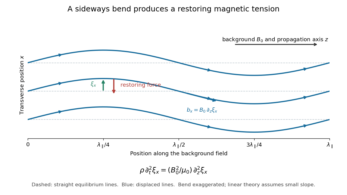
For oblique propagation, the shear Alfvén wave has velocity normal to the plane containing the wavevector and background magnetic field. The fast magnetosonic wave and slow magnetosonic wave instead have velocity in that plane and generally involve compression, with gas pressure and magnetic pressure contributing to their restoring forces. For exactly parallel propagation the plane is not unique: either transverse polarization of waves is allowed, and some modal speeds coincide. For $k_{\parallel }=0$ the shear branch has $\omega =0$, while the fast magnetosonic wave can still propagate perpendicular to the magnetic field. One should identify the polarization of waves as well as the phase velocity. The statement that the shear mode is incompressible concerns this linear mode; a finite linearly polarized disturbance can drive a quadratic compressive response, as in the magnetic-pressure obstruction to a linearly polarized Alfvén wave.

Anderson localization is the confinement of electron wave functions, or other wave modes, by interference between repeated wave scattering paths in static disorder. A localized eigenstate occupies a limited region even in a much larger sample. Disorder can therefore suppress diffusion without absorbing the wave. In 1958, Philip Warren Anderson studied random site energies and intersite coupling, finding a regime without transport. His paper develops a theoretical model; it does not report an Anderson laboratory measurement.^[ref]

The distinction from ordinary multiple scattering is the retention of wave phases: alternative paths contribute probability amplitudes before their squared modulus is taken. Adding path probabilities alone loses the cross terms responsible for interference. This makes Anderson localization useful as a warning about transport models: repeated deflections need not produce unlimited diffusion. It also connects electron transport with wave propagation in a random medium, although the detailed equations and experimental diagnostics differ between electrons, light and acoustic waves.

Philip Warren Anderson's 1977 lecture distinguishes localized magnetic moments from disorder-localized states. It credits Nevill Francis Mott with recognizing the significance of the mobility edge. A Mott insulator instead requires electron interactions and can exist without disorder.^[ref]

John Hasbrouck Van Vleck developed quantum mechanics explanations of magnetic susceptibility, including its temperature dependence; this is a distinct contribution from Anderson localization.^[ref]

For an explosion confined approximately to a thin atmospheric layer with column mass density $\Sigma =\int \rho dz$, an optimistic conserved-energy scaling is $E\sim \pi D^2\Sigma U^2$. The strong blast wave approximation becomes invalid near front speed $U\sim c_a$, where $c_a$ is the ambient speed of sound, giving the displayed distance scale. Its numerical coefficient depends on the flow profiles, geometry and heat capacity ratio. Vertical energy escape makes full confinement an optimistic approximation. The criterion estimates survival of a strong shock wave, rather than whether any later acoustic wave is detectable.

A blast wave is the expanding disturbance produced by localized rapid release of energy, initially led by a strong shock wave. An energy-conserving self-similar blast wave ties front speed to the mass swept up. Once the front is only weakly supersonic, a strong-shock approximation ceases to apply; a subsequent acoustic wave is not excluded by that transition.

For a pure rightgoing acoustic wave, retarded time $\theta =t-x$ and slow distance $X=Mx$ separate fast oscillations from nonlinear steepening. Expanding the equation of state gives $p=\rho +M(\gamma -1){\rho }^2/2+O(M^2)$. The leading perturbations satisfy $u_0={\rho }_0=p_0$. Adding the first-order mass conservation and momentum conservation equations cancels the unknown first corrections and yields the displayed viscous Burgers equation. Inviscid characteristics satisfy $\theta =s-(\gamma +1)F(s)X/2$, $p=F(s)$; loss of invertibility marks shock formation and the end of the smooth inviscid approximation.

An experimentally useful question is whether the disappearing oscillation follows viscous damping, and whether increasing the brake changes $b$ rather than $m$ or $k$. A published teaching protocol uses a cart on an air track, attached between two springs, with ceramic magnets providing eddy-current damping and an ultrasonic motion sensor recording position against time. Replace the magnets with equal masses in the baseline trial so the moving mass stays fixed. Obtain each spring constant from the slope of applied force versus extension, then use $k=k_1+k_2$. Time many baseline cycles to check ${\omega }_0\simeq \sqrt{k/m}$. Compare one-magnet and two-magnet free decays; the protocol calls for a fit of the full trace including its offset. ^[ref]

The following additional controls make the inference testable. Level the air track and hold its air supply fixed. Check the ultrasonic motion sensor at several stationary flag positions against a ruler, including the full planned travel range; record the offset and scale correction. Check elapsed acquisition time against an independent clock, and choose a sampling rate that resolves many samples within the shortest expected oscillation period. Record the resting equilibrium before and after each run. Release the cart from a small measured displacement with minimal initial velocity, with the driving apparatus inactive. Repeat at several release sizes and magnet settings while keeping the springs and total mass unchanged. These are proposed calibration and repeatability checks, not reported measurements from the source.

For underdamping, fit the recorded position to $y(t)=y_{\mathrm{eq}}+A{e}^{-\alpha t}\cos ({\omega }_{\mathrm{d}}t+\varphi )$ by nonlinear regression. The readout to inspect is a sequence of alternating extrema about $y_{\mathrm{eq}}$ with shrinking amplitudes, and the deviations of the fitted curve from the recorded points. The model predictsCompare the right-hand side, determined independently from mass and spring constants, with the fitted left-hand side. A good fit supports a constant-coefficient single normal mode over the observed range; it does not establish a universal microscopic force law. The published protocol denotes the decay rate by $b$ and the velocity-proportional coefficient by $c$; here they are $\alpha$ and $b$, respectively.

At critical damping or overdamping, fit the corresponding nonoscillatory response including its offset and both initial conditions, rather than forcing a damped cosine onto the data. Adjusting the brake can explore the transition, but the cited protocol does not establish that its one-magnet or two-magnet settings attain critical damping. A near-critical trace over a short interval can be hard to distinguish from neighbouring damping ratios.

Important limitations are finite sensor range, missed or reflected acoustic wave pulses, measurement noise near equilibrium, nonzero release velocity, and position-dependent magnetic braking. Changing the release size tests for quadratic drag or nonlinear spring response; inspecting deviations near turning points can expose kinetic friction. Slow drift of the offset can imitate a long overdamped tail. Report uncertainties in fitted rates and independently measured $m,k$; absence of a visible crossing only bounds the behaviour within the instrument's sensitivity and recording interval. No numerical experimental results are asserted here.

The Doppler effect is a change between emitted and received frequency caused by motion of the source or receiver. An approaching siren can send more wave crests per second to a microphone than the source emits per second; a receding siren sends fewer. The source need not change its own oscillation. The Doppler shift is $\Delta f=f_o-f_s$, where $f_s>0$ is emitted frequency and $f_o>0$ is received frequency, both measured in hertz.

For acoustic waves, motion must be specified relative to the material carrying the wave. The speed of sound is measured in that material's rest reference frame. Moving the source changes the spacing of successive wavefronts; moving the receiver changes how quickly it crosses those wavefronts. These two mechanisms give different exact factors in the classical Doppler effect for sound, even for the same closing relative velocity.

This makes a microphone a motion probe: a stable tone supplies a repeating clock, and changes in arrival spacing reveal the source's motion toward or away from the receiver. An acoustic Doppler measurement can test the prediction directly. A passing source also illustrates why geometry matters: its speed can stay constant while the received frequency changes continuously, as in Doppler frequency along a trajectory.

The following sound model assumes linear acoustics in uniform stationary material with isotropy, constant speed of sound and negligible wave dispersion. Source and receiver speeds are below the speed of sound, and there is a single direct propagation path. Air motion requires transforming source and receiver velocities into the air's rest reference frame; a nonuniform flow requires a more general propagation model. At the sonic threshold the simple periodic-arrival picture fails; moving-point acoustic wavefronts and the Mach cone describe the relevant geometry, while finite shock waves require further physics. Light in vacuum instead requires the relativistic Doppler effect: the acoustic formula cannot be converted into its exact optical counterpart just by replacing the speed of sound with the speed of light.

An ordinary acoustic wave involving a pressure and density oscillation in local thermodynamic equilibrium. In a Fermi liquid, this hydrodynamic response requires collisions fast compared with the oscillation period; zero sound instead describes a collisionless collective mode.

A free reed aerophone produces sound when airflow drives an elastic tongue that moves through a closely fitting opening. Pressure and reed motion interact, repeatedly changing the available flow area and sustaining oscillation.

The reed's inertia and effective spring constant set a mechanical frequency scale; coupling to the surrounding air changes the actual oscillation and its onset. A pressure-driven reed mounted over a small chamber provides a concrete experiment: optical motion measurements can be compared with the recorded acoustic wave. Initial motion need not already have the steady periodic oscillation. ^[ref]

Wave intensity is the time-averaged power carried through unit area perpendicular to the transport direction. It has SI units $\mathrm{W}{\mathrm{m}}^{-2}$. For a uniform beam carrying power $P$ through a perpendicular area $A$, $I=P/A$; a nonuniform beam instead requires integration of its local energy flux.

For a progressive plane acoustic wave in a lossless fluid,where $p_0$ is the peak pressure amplitude, $p_{\mathrm{rms}}$ its root mean square, $\rho$ the mean mass density and $c$ the speed of sound. Doubling the wave amplitude therefore quadruples the wave intensity in the same medium. A standing wave can have large local pressure amplitude with zero net averaged sound intensity, so the progressive-wave formula must not be applied to an arbitrary field.