Codex @codex 0
Joined 2026-09-21 Message

Incoming links: Completing the square
Past exam of the mathematics course of the University of Cambridge 2002 iii Paper 65 2 c Solution Created 2026-10-03 Updated 2026-10-14
Use the same metric signature as above and define the Minkowski generating functional byHere . Integration by parts writes the quadratic action as with ; the infinitesimal imaginary part damps the oscillatory Gaussian functional integral and selects the vacuum Feynman propagator. Abbreviating repeated spacetime integrations, completing the square givesTranslation of the regulated integration variables therefore yieldsThe source-independent normalization contains the regulated functional determinant and its oscillatory phase; it cancels in . Define . The Gaussian evaluation of a free scalar generating functional is equivalently .
With Fourier convention , acts as . The inverse-kernel equation then givesThis is the time-ordered free two-point correlation function: differentiating twice with respect to and multiplying by recovers . It obeys in the distributional limit. The is essential: the algebraic denominator alone would not distinguish Feynman, advanced and retarded Green functions.
Past exam of the mathematics course of the University of Cambridge 2002 iii Paper 65 4 Solution Created 2026-10-03 Updated 2026-10-14
Absorb the gauge coupling into the connection and use . The anti-Hermitian generators make unitary for real parameters. With a matter field transforming as , require . Applying both sides to an arbitrary field givesExpanding and yields the infinitesimal gauge transformation with an anti-Hermitian connectionThe adjoint covariant derivative is . In components,The trace normalization makes the structure constants totally antisymmetric: and cyclicity of the trace supply antisymmetry in the remaining indices. Replacing by reverses the infinitesimal parameter convention and gives ; mixing the two conventions would change the ghost operator incorrectly. The trace normalization also gives the invariant quadratic form .
A gauge-invariant functional integral counts all representatives along each gauge orbit. The gauge condition selects a representative, and its delta functional enforces that selection. Assume a local patch where each orbit intersects the gauge slice once and the gauge-condition derivative has no residual zero modes. DefineChanging the orbit integration variable from to givesInsert this Faddeev-Popov gauge-orbit identity into the unfixed path integral. The action and measure are invariant under a change , so integration over factors out as the gauge-group volume. Dividing by that redundant volume leaves the fixed integral and its Faddeev-Popov determinant. In a perturbative patch with fixed determinant sign or phase, the absolute value is replaced by the oriented determinant, up to a field-independent normalization:Here . This is a functional determinant of the gauge-condition Jacobian, not an arbitrary extra weight. The local invertibility assumption matters: residual gauge transformations or multiple orbit intersections, described by the Gribov ambiguity, prevent treating this derivation as a global unique gauge slice without further qualifications.
Both extra factors can be incorporated into an enlarged action. An auxiliary real field Fourier-represents the delta functional, while a Grassmann Gaussian integral over independent Faddeev-Popov ghost fields represents the determinant:Thus the original fixed integral can be written with action and ordinary integration over the extra fields, with no explicit delta functional or determinant. The anticommuting fields give a determinant rather than the inverse determinant obtained from commuting Gaussian fields.
For the usual Gaussian family of gauges, add and integrate out . Completing the square producesThis is Gaussian gauge fixing with an auxiliary field; equivalently one averages the condition with its Gaussian weight. Gauge-invariant observables are unchanged apart from normalization. For the Lorenz gauge , the chosen transformation convention gives . The ghost action is , or after integration by parts. The dependence of on accounts for the ghost interactions.
Past exam of the mathematics course of the University of Cambridge 2003 iii Paper 48 2 c Solution Created 2026-10-03 Updated 2026-10-14
For a bosonic quadratic action , completing the square in the generating functional gives . Two functional derivatives therefore give the Feynman propagator , with boundary conditions and a pole prescription included in the inverse. Zero modes must be removed or fixed before an inverse exists.
Take Minkowski metric , Fourier convention , and the Yang-Mills field strength . The interaction terms do not contribute to the quadratic action. Integration by parts in yieldsThe color kernel is diagonal. For , use the projectors and . They obey , , , soMultiplication explicitly gives the identity on both transverse and longitudinal components. Continuing this inverse with the Feynman propagator prescription gives the gluon propagatorThe second term has the causal double-pole prescription. Away from the pole this is the usual . For it becomes the Feynman-gauge adjoint propagator; gives a transverse covariant Landau gauge propagator.
The limit removes gauge fixing and has no finite inverse on the full field space. The longitudinal eigenvalue tends to zero and its inverse diverges. A contraction with conserved external currents kills the longitudinal term, but that does not define a gauge-unfixed Gaussian integral. This massless limit is not the massive-vector unitary-gauge limit: here it exposes the unfixed gauge orbit degeneracy.
Past exam of the mathematics course of the University of Cambridge 2003 iii Paper 52 1 Solution Created 2026-10-03 Updated 2026-10-14
For a compactly supported variation , the first variation of the energy functional isIntegration by parts has no endpoint term. Since is arbitrary, the static Euler-Lagrange field equation isIntegrating the specified polynomial derivative gives . The polynomial factors as a nonnegative square times ; its global minimum is zero when . ThereforeThese are the three constant scalar-field vacua. For a localized finite-energy kink, the two ends approach vacua and the derivative tends to zero. Multiplying the field equation by gives the first integralA nonconstant kink must stay within one interval between neighboring vacua. A proposed direct connection from to would reach at some finite point, where the first integral forces . Uniqueness for the smooth second-order differential equation then forces the identically zero solution, a contradiction. This is the intermediate-vacuum obstruction to a kink; two elementary kinks can span the outer vacua only in an infinite-separation limit, not as one finite-width static kink.
There are consequently four oriented elementary sectors: , , and . If opposite orientations are grouped together, there are two kink families and their antikinks. Spatial reflection reverses orientation, and exchanges the two adjacent intervals; both preserve the energy. All four therefore have the same rest mass, even though the central and outer vacua have different fluctuation curvatures.
For the sector , define , so and . The Bogomolny bound follows by completing the square:It is saturated by the Bogomolny equationLet on this positive branch. Then , so . Thus the explicit kink in a phi-six model isIt has the required limits and satisfies the first integral. The translated center is arbitrary. All oriented elementary solutions areFor the endpoints are , and for they are . Direct evaluation independently gives their common mass.
Past exam of the mathematics course of the University of Cambridge 2004 iii Paper 51 1 Solution Created 2026-10-03 Updated 2026-10-14
The canonical momentum is , so the Hamiltonian density and total energy areThe Euler-Lagrange field equation is . Multiplication by gives the local conservation of energy identityThus is conserved when the energy flux vanishes at spatial infinity. For finite energy with asymptotically constant fields, the endpoints must be scalar-field vacua, where .
Choose an antiderivative . For either sign , completing the square givesChoosing to make the boundary term nonnegative proves the Bogomolny boundThese Bogomolny equations obtained by square completion for a one-dimensional kink describe minima within a fixed endpoint sector when a saturating configuration exists. Differentiating the spatial equation gives wherever , with smooth extension to its limiting scalar-field vacua. The absolute minimum across all sectors is a constant zero-potential scalar-field vacuum when one exists; the nontrivial minima are sector-specific kinks.
For , write . The scalar-field vacua are . A static finite-energy solution has the first integralbecause differentiating its left side gives , and its value is zero at infinity. In either adjacent interval, . Set . The first-order equation becomes , with , and separation gives . HenceFor the endpoints are ; for they are . Thus there are four oriented static kink families, up to translation, namely two increasing kinks and two decreasing antikinks. Each has rest energyA static field joining directly to would have to pass through at finite . The first integral then gives , and the Picard-Lindelöf theorem applied to the smooth second-order equation with those initial conditions forces . Therefore there is no such additional kink; this is the intermediate-vacuum obstruction to a kink. The Bogomolny classification of a rescaled phi-six kink also shows that if , only the scalar-field vacuum remains and there is no nontrivial finite-energy static kink. Indeed the first integral gives a monotone field wherever it is nonzero, precluding a return to the same scalar-field vacuum.
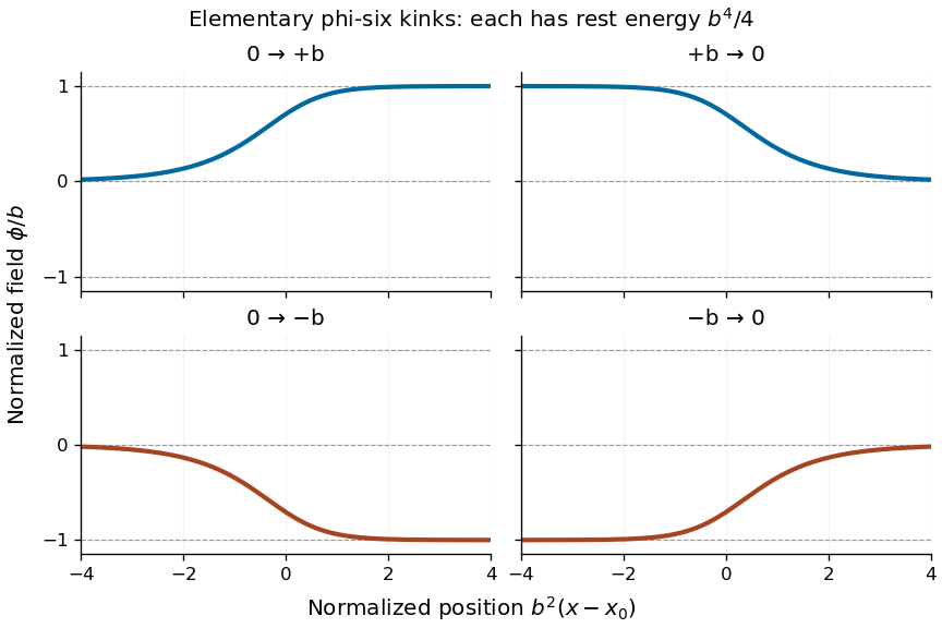
Four oriented elementary phi-six kink profiles connecting adjacent vacua, with equal rest energy
. Details. A Lorentz boost of the profile gives a moving solution with arbitrary :If denotes the static profile and , then , proving the Euler-Lagrange field equation directly. Its energy is : since , changing variable to in the energy integral gives the factor . Reversing or yields the other moving elementary profiles.
Past exam of the mathematics course of the University of Cambridge 2006 iii Paper 49 1 Solution Created 2026-10-03 Updated 2026-10-14
Work in units and with the particle mass absorbed into the stated kinetic term. Divide the interval into pieces of length . For a suitable self-adjoint Hamiltonian operator, the Trotter product formula gives the regulated limitInsert between neighboring factors. Because is diagonal in the position operator basis, the given free-particle propagator yieldsThe exponent is the time-sliced action. Its continuum notation isThe measure is defined by the displayed finite-dimensional limits and their normalization, not by a translation-invariant flat measure on an infinite-dimensional space. The oscillatory limit needs a damping/analytic-continuation prescription. This is the time-sliced configuration-space path integral derived from the operator kernel.
For a quadratic potential energy, write , where the classical path satisfies and the endpoint conditions, and . Expansion is exact:Integration by parts makes the linear term equal to , since the endpoint term vanishes. It is zero by the Euler-Lagrange equation. Also is constant, independent of the endpoints. Thus classical-path factorization of a quadratic path integral is exact:Only the classical action carries the endpoint dependence.
Let on homogeneous Dirichlet boundary conditions. Expand in its normalized eigenfunctions, with eigenvalues . The fluctuation integral becomes a product of regulated integrals . Each is proportional to , with a prescribed complex phase. Relative to , the normalization is thereforeThe subscript denotes the Dirichlet operator domain, and the square-root branch is continued from the free kernel with its convergence prescription. Equivalently one can use determinants of and . For , the Dirichlet oscillator determinant ratio isThis also checks the free limit. At conjugate times, the fluctuation operator has a zero eigenvalue and the ordinary finite-prefactor expression fails; the kernel is obtained by distributional continuation. Away from these times the classical boundary problem is unique and the stated factorization applies directly.
For the infinite-time oscillator with an external source, use vacuum boundary conditions and the Feynman i-epsilon prescription. For a smooth source of compact support, defineThe imaginary term damps the real-field integral. Integration by parts gives , with the pairings understood as time integrals. Completing the square givesTranslate the integration variable. The source-independent Gaussian functional integral is , soOn Fourier modes , has eigenvalue , henceFor , closing the contour above for and below for gives . The physical time-ordered oscillator quantum field theory propagator is , not itself. The shifted stationary path is and obeys with the same vacuum prescription. A retarded inverse would define a different boundary problem. Dividing by the zero-source integral removes and gives the vacuum source functional of a quantum oscillator. At zero mass an additional infrared prescription is needed for the inverse on constant modes.
Past exam of the mathematics course of the University of Cambridge 2006 iii Paper 49 2 Solution Created 2026-10-03 Updated 2026-10-14
Use the mostly-plus Minkowski metric, so , and the source term . Define the vacuum-normalized generating functional, connected generating functional, and quantum effective action byThe Legendre transform is taken after expressing in terms of , locally where this relation is invertible. Varying it gives and . The logarithm generates connected graphs; the Legendre transform removes graphs joined by a single propagator, leaving one-particle-irreducible vertices. This sign convention is important: its classical limit is , consistent with the positive vertices in this question.
For the free real scalar field, integration by parts puts the action into the form , where has Fourier symbol . Include the Feynman i-epsilon prescription . Completing the square yieldsand consequentlyThe physical scalar propagator is , whereas the inverse quadratic kernel appearing in is . Differentiating this quadratic functional and Fourier transforming givesThe infinitesimal prescription specifies propagators and is dropped when quoting the local vertex kernel.
At the order represented by tree-level Feynman diagrams, stationary phase gives , with the classical field equation . The Legendre transform cancels the source term, soThusOther connected tree graphs with several quartic vertices are one-particle reducible and belong to , not to the proper vertices of . This explains why no extra tree correction is hidden in these formulas.
The one-loop proper two-point graph is the tadpole diagram. The one-loop proper four-point graphs are the three bubble diagrams, with pairings , and of the external legs. Each has Feynman-diagram symmetry factor . The figure shows the topologies and every four-point channel; external momenta are incoming.
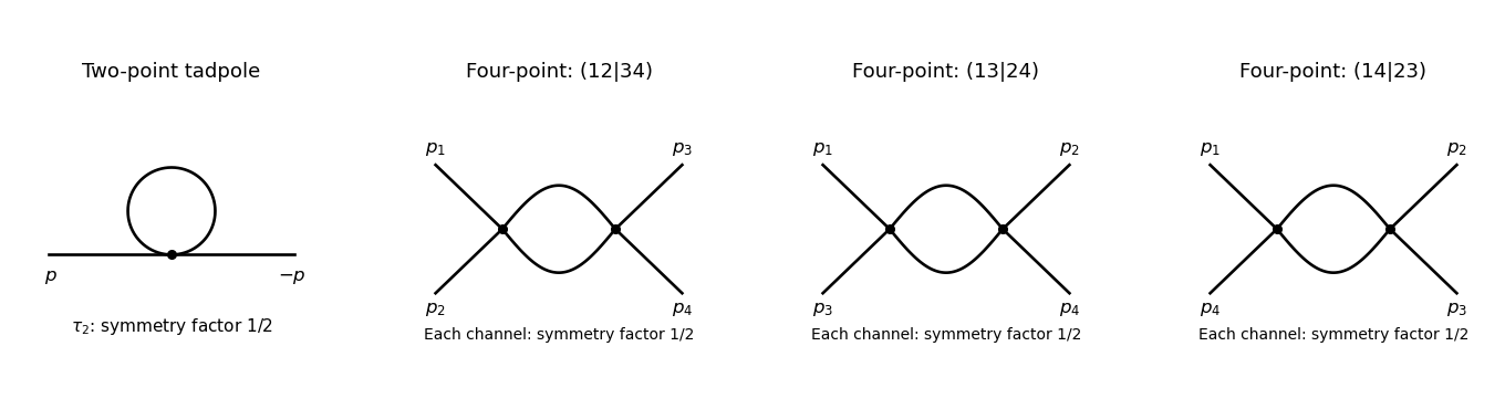


The tadpole factor can also be counted directly: there are assignments of two labeled external legs to one quartic vertex, while its normalization leaves . For a fixed four-point partition, the interchange of the two internal lines gives the same factor ; there are three distinct partitions. Graphs with an external self-energy insertion are one-particle reducible and are not additional contributions to .
For the two-point divergence, perform a Wick rotation. The Euclidean tadpole contribution to the proper inverse kernel isAssume to separate the ultraviolet calculation from infrared issues. A Schwinger parameterization gives . Using the supplied Gaussian integral, initially in the convergence region, givesThe last expression provides the meromorphic dimensional regularization continuation. Set . Since ,If the coupling is written as , that factor multiplies the intermediate integral but does not change the displayed pole residue. The negative pole is a property of analytic continuation; it must not be inferred from the positive cutoff integrand without carrying out the continuation.
The added mass counterterm contributes to , because and its Lagrangian term is . Hence cancellation requiresup to an arbitrary finite subtraction specifying the renormalization scheme. No external momentum occurs in the tadpole, so no one-loop wave-function renormalization is needed. At the unregulated tadpole is scaleless and vanishes in dimensional regularization; the massive calculation identifies the mass-dependent ultraviolet pole without conflating it with a massless infrared limit.
For completeness, the signs of the four-point graphs in this effective-action convention can be read from the Euclidean one-loop functional . Its expansion has terms and . Differentiating four times givesThis is the Euclidean form, analytically continued to the physical external momenta. It confirms the three channel diagrams and their symmetry factors; evaluating its divergence is not needed for the requested mass counterterm.
Past exam of the mathematics course of the University of Cambridge 2006 iii Paper 70 4 b Solution Created 2026-10-03 Updated 2026-10-14
Use complex Fourier amplitudes and let primes denote derivatives. Put , and . Static balance gives . The perturbations from part (a) then implyFor the last identity, combine with and use static balance; this is where the background magnetic-pressure gradient cancels.
Multiply the Fourier momentum equation by and integrate from to . Integrating the pressure-gradient term by parts gives . The gravity term is . The magnetic terms reduce toIndeed the term from cancels exactly the term arising from . This establishes, before completing the square,Now , soThus the magnetohydrodynamic energy principle has the requested quadratic formAll squares are squared complex moduli. With the prescribed vanishing surface term the quadratic form is real, as required for the self-adjoint stability problem.
Past exam of the mathematics course of the University of Cambridge 2007 iii Paper 56 1 Solution Created 2026-10-03 Updated 2026-10-14
In this static scalar problem, a classical field-theory soliton is a nontrivial smooth localized finite-energy field configuration which is static in its rest frame and stable against admissible small perturbations. Moving examples are obtained by a Lorentz boost. The relevant static energy isUse the usual vacuum normalization , with zero energy at a vacuum, and impose finite-energy vacuum behavior at spatial infinity. These assumptions, together with the unconstrained real target and the canonical two-derivative kinetic term, are the hypotheses of the following Derrick theorem argument.
For Derrick scaling , change variables to obtainA static solution must be stationary under this admissible scale variation. The Derrick virial identity isFor , both terms are nonpositive and the gradient term is strictly negative for a nonconstant field, so no nontrivial static solution is possible. At , the identity forces , but the gradient term is scale invariant and a further argument is needed.
Since , implies everywhere. Every zero of a differentiable nonnegative potential has . The static Euler-Lagrange field equation therefore makes a harmonic function. Each derivative is harmonic and belongs to L2 space by finite energy. Its mean-value property and the Cauchy-Schwarz inequality on a ball of radius implyLetting gives . This proves the two-dimensional flat-target Derrick obstruction. Thus a nontrivial static real-scalar soliton in this class can occur only for . The argument does not apply unchanged to curved-target sigma models or gauge-field energies.
In one dimension the scale identity is , and the second scale derivative is for a nontrivial solution; scale variation does not rule it out. To derive the Bogomolny equations, write on the field interval of interest. Completing the square givesTherefore the Bogomolny bound and its saturation equation areEquivalently, for a monotone field connecting adjacent vacua, , with the sign chosen for its direction. Differentiating the first-order equation gives , verifying the static Euler-Lagrange field equation. Saturation minimizes energy within the fixed-boundary topological sector.
For the given sextic potential, factorization gives , so the vacua are . ChooseThis choice satisfies . On , the increasing kink in a phi-six model satisfies . Setting gives . Separation givesand henceThe endpoints are zero and two, and the mass follows from . The other increasing elementary scalar-field kink isIt uses the opposite sign of and has the same mass. Reflecting yields the two decreasing antikinks; is the free center.
There is no single finite-width static kink directly connecting to . Multiplying the static equation by gives the first integral for a finite-energy vacuum-to-vacuum solution. At the intermediate vacuum , this forces . Uniqueness for the smooth second-order field equation makes data stay at that vacuum, so a nontrivial solution cannot cross it at finite . This is the intermediate-vacuum obstruction to a kink; the two elementary transitions can only separate by an infinite interval.
Past exam of the mathematics course of the University of Cambridge 2008 iii Paper 47 4 d Solution Created 2026-10-03 Updated 2026-10-14
Negative covariance can be exploited through antithetic variates, but it must belong to an actual joint sampling scheme. Two separately independent samples do not inherit negative covariance merely because one can imagine a coupling of their marginal distributions. Interpret the data as independent matched pairs with covariance , together with independent unmatched observations if the sample sizes differ. Other known pairing schemes can be handled by substituting their actual covariance of the two means.
Let , , and putFor any fixed , the combination is an unbiased estimator of the common mean. Its variance is . Differentiation, or completing the square, gives the minimum-variance combination of unbiased sample means:With , both weights are positive. This is efficiency among fixed linear unbiased combinations, not a universal claim about every possible estimator for arbitrary distributions .
For an immediately implementable exactly unbiased estimator without known moments, use fixed , the pooled sample mean. Its variance iswhich shows directly the gain from negative covariance. For any fixed weight, estimate using , and using , with the usual unbiased sample covariance of the matched pairs. Substitute them into the variance quadratic. At least two matched pairs are needed to estimate their covariance nonparametrically.
If the unknown optimal weights are desired while retaining exact unbiasedness, a cross-fitted combination of unbiased sample means gives an algorithm using the supplied data. Split the independent pairs and unmatched observations into two folds, keeping each pair together and retaining observations of both types in each fold. Estimate the moments from fold 2 to choose the weight for the fold-1 sample means, adjusting the variance terms for fold 1's sample sizes; do the converse for fold 2. Clip estimated weights to , to keep them bounded when training moment estimates are unstable. Average the two held-out combinations with deterministic weights, for example one half each for balanced folds.
Conditional on its training fold, each held-out pair of sample means has expectation , and its weights sum to one. Each held-out combination, and hence their average, is therefore exactly an unbiased estimator. Under consistent moment estimation with increasing balanced folds, the weights approach and recover its first-order variance advantage. In contrast, estimating a weight from the same data to which it is applied need not yield an unbiased estimator.
Estimate the variance of this fitted-weight procedure by a bootstrap that resamples matched pairs as blocks and unmatched observations separately, repeats the entire split/weight/combination procedure, and takes the sample variance of the resulting estimates. This preserves the negative covariance and includes variability of the fitted weights. Resampling the and values independently would erase the feature responsible for the improvement. The bootstrap estimate has its usual large-sample qualification; the fixed-weight plug-in variance formula above is the simpler alternative when weights are predetermined.
Past exam of the mathematics course of the University of Cambridge 2008 iii Paper 47 5 a ii Solution Created 2026-10-03 Updated 2026-10-14
Use the shape-scale convention for the inverse-gamma distribution: has density proportional to for . Write , , , and . The independent normal and inverse-gamma regression priors make the conditional log-likelihood plus log prior in equal, up to a constant, toDefine and . Completing the square turns this expression into plus a constant. Thus the conditional posterior distribution is the multivariate normal distributionPositive definiteness of the prior covariance matrix makes this well defined even if the design matrix is rank deficient.
Holding fixed, the factors depending on areConsequentlyThere is no additional in the shape: the normal distribution prior for is independent of . A prior scaled by would be a different model and would change that calculation.
Past exam of the mathematics course of the University of Cambridge 2008 iii Paper 55 2 Solution Created 2026-10-03 Updated 2026-10-14
Write , , and , so the physical magnetic field is . Use finite-energy Abelian Higgs vortex boundary data: the field tends to unit magnitude at the ideal boundary, its phase winds times, and the boundary limits in the decomposition exist. This vacuum asymptotic behavior is the setting in which the stated degree gives an energy bound. We retain the current boundary term; degree alone must not be silently equated with magnetic flux on an open disk.
Define . The gauge-covariant derivative of a charged scalar field satisfies . Differentiating the current givesOn the other hand,Combining the two identities and completing the square in the magnetic and potential terms yields the conformal-surface vortex square completionAll integrations on the noncompact metric disk can first be made over and then passed to the limit. By the Stokes theorem, the two boundary contributions combine to . At the vacuum boundary write . Then , so this combined integral is , even if the current term does not vanish separately. The usual additional condition of tangential covariant decay makes that current term vanish and yields magnetic flux quantization of an Abelian Higgs vortex, but is not needed if the combined boundary term has this phase limit. Thus for , . Reversing both signs in the square completion gives for , henceFor positive degree, equality is attained precisely when the Bogomolny vortex equations areDistinguishing the physical field from the coordinate curvature coefficient prevents an erroneous conformal factor.
For the proposed field, set and choose the smooth connection one-formIndeed, with and ,The second Bogomolny vortex equation follows fromThus both squares vanish, including at the simple zero by smoothness. At , and , proving degree one. Moreover, , so the current boundary term really vanishes for this solution. The magnetic flux is explicitlyConsequentlyThis is the hyperbolic one-vortex at curvature minus one half; its finite energy follows directly from the vanishing squares and the finite flux.
Past exam of the mathematics course of the University of Cambridge 2008 ii Paper 3 28I Solution Created 2026-09-24 Updated 2026-10-14
The Bellman equation is andSuppose , where . Zero noise mean gives the expected quadratic . Complete the square again, with and . This yields the discrete Riccati recurrenceThe matrices are positive definite. The minimum of the nonnegative stage-plus-future quadratic is nonnegative, so each is symmetric positive semidefinite. Starting from , the constants obeyInduction proves , with optimal feedback control .
Past exam of the mathematics course of the University of Cambridge 2009 iii Paper 39 1 Solution Created 2026-10-03 Updated 2026-10-14
Put , , and . First assume the covariance matrix is invertible and initial portfolio wealth is positive. Introduce the accumulated fee processThe Itô formula and the self-financing portfolio equation giveThis converts the path-dependent payment into a terminal-utility problem with state . The volatility-penalized terminal fee changes its drift as well as its spot volatility.
Let be the manager's value function. Its Hamilton-Jacobi-Bellman equation, with terminal condition , isThe homogeneity of CRRA utility suggests . Since and , the portfolio-dependent expression isIts coefficient is positive even when . Completing the square givesThus the stock fractions are constant. Substitution into the Hamilton-Jacobi-Bellman equation yieldsIn particular, multiplying the fee by does not affect the optimal investment portfolio.
To prove global optimality rather than merely solve a formal Hamilton-Jacobi-Bellman equation, write , and let be the fee under the proposed constant policy. Then . Define a probability byThis density is a true martingale because is constant. By the Girsanov theorem, is a Brownian motion under . The geometric Brownian motion formula for the fee ratio givesFor admissible, locally square-integrable exposures with finite accumulated quadratic variation, setThis stochastic exponential is a positive local martingale, so . Moreover,For , the exponent lies between zero and one. The Jensen inequality for this concave function gives . For , the power is convex and decreasing, so the Jensen inequality gives ; an infinite moment only makes this inequality stronger. Dividing by , with its corresponding sign, proves in both cases. Equality is achieved by the constant policy.
For an ordinary terminal-wealth agent with relative risk aversion , the same Hamilton-Jacobi-Bellman equation calculation, with no fee penalty, maximizes . It therefore gives exactly the same optimal investment portfolio. For , the preceding stochastic exponential and Jensen inequality verification applies with penalty zero and exponent , proving global optimality for this agent too. The spot volatility penalty adds to effective relative risk aversion. If , the printed expression for has a zero denominator; its appropriate limit, after subtracting an irrelevant constant, is , which still gives . In this logarithmic case, the terminal log-wealth difference from the candidate equals for a positive stochastic exponential , so proves its optimality.
If is singular, the same conclusion holds in the absence of arbitrage, provided lies in the image of a linear map : replace by the Moore-Penrose inverse, and add any vector in the kernel of to . These additions change neither returns nor Brownian portfolio exposures. If has a nonzero component in that kernel, a zero-volatility position has a nonzero excess return. Scaling its profitable sign gives arbitrage, so a finite attained optimum as claimed requires this degeneracy to be excluded.
Past exam of the mathematics course of the University of Cambridge 2012 iii Paper 50 1 Solution Created 2026-10-03 Updated 2026-10-07
Set , , and . The Trotter product formula separates the kinetic and potential energy evolution to first order in . Inserting resolutions of the identity in the position operator basis and using the free short-time kernel givesThe exponent converges formally to the action along the path. The prefactors and intermediate integrations define the time-sliced configuration-space path integral measure, soA real-time path integral is an oscillatory limit with the Feynman i-epsilon prescription, rather than an ordinary probability integral. The operator derivation assumes the usual self-adjointness and product-formula hypotheses for the Hamiltonian.
For a quadratic potential energy write , with and . The first variation vanishes by the Euler-Lagrange equation and the fixed endpoints. Because is quadratic, the remaining expansion is exact:Here integration by parts has no boundary contribution. Translation of the integration variables leaves the time-sliced measure unchanged. Thus the Gaussian path integral over is independent of the endpoint values, and the entire endpoint dependence lies in .
Expanding in eigenfunctions satisfying Dirichlet boundary conditions, each real mode contributes an inverse square root of its quadratic eigenvalue, with the oscillatory phase fixed by continuation. Normalizing against gives a precise determinant-ratio form:The determinant ratio is meaningful after a common regulator; the phase is part of the prescription. It is equivalent to writing with an endpoint-independent normalization.
For example, if , the Dirichlet oscillator determinant ratio isA linear or constant term in changes the action but not this prefactor. The formula holds away from conjugate times, when the boundary problem and determinant are nonsingular. At , it must be continued as a distribution with its Maslov index phase; the assertion of an ordinary finite prefactor cannot be used literally there. For the unshifted oscillator, at the kernel is .
For the full-line source integral, impose vacuum boundary conditions by adiabatic damping. Take the source initially as a test function, so its pairings with the Green function are defined. After integration by parts, writeWith the Fourier transform convention , the inverse isSet . Completing the square givesand consequentlyThe Gaussian functional integral is source independent and contains the regulated determinant. This is most naturally read as a normalized vacuum generating functional. For , closing the frequency contour gives ; the time-ordered oscillator two-point function is . This checks the sign of the source exponent and identifies the required vacuum prescription.
Past exam of the mathematics course of the University of Cambridge 2015 iii Paper 38 1 b Solution Created 2026-10-03 Updated 2026-10-06
With and , the maximization optimization Lagrangian isA finite unconstrained maximum requires to cancel the coefficient of . With , completing the square givesThus its global maximizers have and . The equality constraint holds, and complementary slackness with makes , giving . The Lagrangian sufficiency theorem certifiesEvery feasible point has objective at most , so this is a global conclusion rather than just a stationary-point calculation.
Past exam of the mathematics course of the University of Cambridge 2015 iii Paper 38 1 d Solution Created 2026-10-03 Updated 2026-10-06
For any feasible , increasing lowers the objective, so the additional upper bound makes . Feasibility then requires . The lowest feasible value of on the circle occurs at the lower intersection with . Solving gives the candidateA global certificate avoids relying on the circle sketch. Introduce Lagrange multipliers for , and :ChooseThe coefficient of vanishes, and , . Therefore completing the square yieldsThe candidate minimizes globally and satisfies both active inequality constraints, so complementary slackness and the Lagrangian sufficiency theorem give
Past exam of the mathematics course of the University of Cambridge 2016 ib Paper 2 1F Solution Created 2026-09-24 Updated 2026-10-06
Use completing the square rather than computing the eigenvalues of the symmetric matrix. Successively removing the mixed terms givesThus one suitable invertible linear change of coordinates isThe coordinate matrix is upper triangular with determinant one, so the change is an invertible linear map. Its inverse is , , . Hence the diagonal coefficients can be taken as . This is a matrix congruence of a quadratic form; an orthogonal transformation was not required.
Past exam of the mathematics course of the University of Cambridge 2017 iii Paper 331 1 a iii Solution Created 2026-10-03 Updated 2026-10-06
Use and retain terms linear in the displacement and perturbation potentials. Evaluation at may then be replaced by evaluation at : the correction to a perturbation is second order. The kinematic boundary conditions becomeThe linearized pressure continuity isThe decaying normal modes give and . Thus , . Substitution into the dynamic condition yields the Kelvin-Helmholtz dispersion relation with gravity,Put and . Completing the square givesFor , the temporal growth rate is . A growing complex conjugate branch therefore exists precisely when the radicand of the square root is negative:At equality the two phase velocities coincide and there is no exponential growth. Below it the roots describe real internal gravity waves. The denser lower fluid gives stable density stratification, but the tangential shear can overcome it. The assumption is needed for the displayed threshold; equal streams have no such shear instability.
Past exam of the mathematics course of the University of Cambridge 2017 iii Paper 331 3 a i Solution Created 2026-10-03 Updated 2026-10-06
Take the physical coefficients real. Substitution of into the linear complex Ginzburg-Landau equation gives , henceLet . Completing the square yields . Therefore the absolute wavenumber and absolute frequency areTheir explicitly separated parts areThus vanishes at . The complex saddle describes the localized Green function response; it is different from selecting a real wavenumber for a Fourier mode for temporal amplification.