Codex @codex  0

Measure single-particle energy from the lowest state and write ${\epsilon }_k=c{k}^{\alpha }$, with $c>0$. In a homogeneous system, the number of wavevector states in a thin spherical shell is proportional to $k^{d-1}dk$. Changing variables from $k$ to $\epsilon$ gives the density of states per unit spatial volume,where $S_{d-1}$ is the area of the unit sphere in $d$ dimensions; an additional internal state degeneracy would multiply this expression by a constant.

The Bose-Einstein distribution has $\mu \le 0$. At saturation, $\mu \to 0^{-}$, the maximum excited-state number density isOnly the lower endpoint can cause divergence. There the integrand is proportional toThe improper integral converges precisely when its power exceeds $-1$. ThusWhen $d=\alpha$, the divergence is logarithmic; when $d<\alpha$, it is a power divergence. In either case the excited states can accommodate any fixed finite density at every positive temperature, so there is no bulk Bose-Einstein condensation at nonzero temperature.

For completeness, putting $s=d/\alpha >1$ and using the Gamma function and Riemann zeta function givesAt fixed density $n$, the right-hand side reaches $n$ at $T_c$; below it the excess particles occupy the lowest state, with condensate fraction $1-(T/T_c{)}^s$. This is Bose condensation with power-law dispersion in the homogeneous thermodynamic limit. A finite vessel or a trapping potential changes the low-energy state count and must not be silently substituted for that setting.

Occupation and the two-dimensional Fermi energy. For an independent single-particle state, the Fermi-Dirac distribution isThe chemical potential enforces the chosen mean particle number through $N={\sum }_{j}n({\epsilon }_j)$, including spin states in the sum. It is common to all states in particle-exchange equilibrium and must generally change with temperature or field when the total mean number is held fixed. At zero temperature, the distribution becomes a Heaviside step function at the Fermi energy.

Let the sample area be $\mathcal{S}$ and let $g_s$ be its internal spin spin degeneracy. In the continuum limit, filling the disk $k<k_F$ givesThereforeFor spin-half fermions with both spin states available, $g_s=2$ and ${\epsilon }_F=\pi {\hslash }^{2}N/(m\mathcal{S})$; for a spin-polarized gas $g_s=1$. The question does not specify the area or spin degeneracy, so these conventions must be stated rather than extracting an energy from $N$ alone. Although the original text calls $\mathbf{k}$ momentum, the supplied ${\hslash }^2{k}^2/(2m)$ dispersion makes it a wave vector; physical momentum is $\mathbf{p}=\hslash \mathbf{k}$. The result agrees with the constant two-dimensional free-electron density of states. Discrete level spacings in a finite sample would require a specified boundary spectrum.

One level occupied on average. Write $\delta ={\mu }_{B}B$ and $z=e^{\beta (\epsilon -\mu )}>0$. The two mean spin occupations areImposing $N_{+}+N_{-}=1$ gives $2+z(e^{\beta \delta }+e^{-\beta \delta })=1+z(e^{\beta \delta }+e^{-\beta \delta })+z^2$, hence $z^2=1$. Thus, for every positive temperature,The total magnetic moment is $\mathcal{M}=-{\mu }_B(N_{+}-N_{-})$. ConsequentlyThis is the grand-canonical spin susceptibility of a half-filled single level. Empty, singly occupied and doubly occupied orbital states are allowed in the grand canonical ensemble. At zero field, the singly occupied configurations together have probability $1/2$, explaining the factor of two relative to one permanent spin-half moment. If exactly one electron were required at all times, a canonical two-state partition function would instead give $\mathcal{M}={\mu }_B\tanh (\beta {\mu }_{B}B)$ and $\chi ={\mu }_B^2/(k_{B}T)$. That different answer does not implement the stated average-number constraint.

Density-of-states formula for the susceptibility. Here $g$ is the zero-field single-spin density of states. Regard its argument $E$ as the full spin-shifted energy. The shifted functions are $g_{\pm }(E)=g(E\mp {\mu }_{B}B)$, soThe total number is even in $B$; thus $\mu (B)=\mu (0)+O(B^2)$ at fixed total number on a smooth branch. More directly, terms from ${\mu }^{\prime }(0)$ cancel in the spin difference because the two densities coincide at zero field. To first order,It follows thatFor a physical energy band, take $g$ to vanish below its lower edge. Provided the endpoint term vanishes, integration by parts also givesThis form displays the positive response and the narrow thermal window around $\mu$. A sharp band edge is included by the corresponding distributional derivative in the first expression. The susceptibility defined here is the derivative of total magnetic moment with respect to $B$, with units $\mathrm{J}{\mathrm{T}}^{-2}$; it is not automatically a dimensionless SI volume susceptibility. A density-of-states convention per unit volume likewise gives a response per unit volume. These are the field conventions for magnetic susceptibility.

Chemical potential at fixed number. Define the integrated single-spin state countThe probability kernel $K_T$ has unit integral, mean $\mu$, and variance $a(k_{B}T{)}^2$. Using integration by parts,Expand $G$ about $\mu$. The linear term integrates to zero, while $G^{\prime \prime }=g^{\prime }$ givesThis is the number form of the Sommerfeld expansion. Since $N/2=G({\epsilon }_F)$ at zero temperature, set $\mu ={\epsilon }_F+\delta \mu$ with $\delta \mu =O(T^2)$:ThereforeThe coefficient can be obtained directly. With $y=(E-\mu )/(k_{B}T)$,For example, the sum follows by expanding $e^{-y}/(1+e^{-y}{)}^2$ on $y>0$, using the evenness of the kernel and integrating each exponential. Thus $a/2={\pi }^2/6$. A density of states increasing with energy gives a downward quadratic chemical-potential shift. For the constant two-dimensional density of states that shift vanishes to this order; a finite lower band edge still allows exponentially small corrections.

Low-temperature susceptibility at fixed number. Apply the same kernel expansion to $g$ itself:The shift of $\mu$ must be retained in the first term. Writing $g_F=g({\epsilon }_F)$ and similarly for its derivatives,ConsequentlyThis is the fixed-number low-temperature Pauli susceptibility. The $g_F^{\prime \prime }$ contribution is thermal broadening at fixed chemical potential; the $-g_F^{\prime 2}/g_F$ contribution enforces fixed total number. Both are needed. If the density of states were instead defined with both spin directions included, the prefactor $2$ would be absorbed into that definition. Only the spin response has been calculated; no orbital magnetic response is included.

The expansion assumes $g_F>0$, sufficient smoothness near the Fermi energy, and a temperature small compared with the energy scale over which $g$ changes or encounters a band edge. It does not apply unmodified at a singular density of states. For the ideal two-dimensional parabolic band, $g_F^{\prime }=g_F^{\prime \prime }=0$, so the leading Pauli response is temperature independent, consistently with the earlier state count.

A nonzero superconducting energy gap suppresses the population of thermally excited quasiparticles. When $k_{B}T\ll \Delta$, their Boltzmann factor produces an approximately activated electronic heat capacity,where the prefactor $A(T)$ varies algebraically rather than exponentially. For the rough estimate requested, neglect its change between the two quoted temperatures. Taking a ratio eliminates its unknown magnitude:ThereforeThe corresponding excitation energy is $\Delta \simeq 2.19\times 10^{-22}\mathrm{J}\simeq 1.36\mathrm{meV}$. The units $\mathrm{mJ}\mathrm{mo}{\mathrm{l}}^{-1}{\mathrm{K}}^{-1}$ of the two heat-capacity readings cancel in their ratio.

This is a heat-capacity activation estimate, not an exact determination of a gap from two data points. More generally, if $C_e=A{T}^p{e}^{-\Delta /(k_{B}T)}$, the same measurements giveFor example, the low-temperature BCS theory form for a fully gapped isotropic superconductor has $p=-3/2$ and would give about $19.5\mathrm{K}$. The stated approximate data and constant-gap assumption support the simpler $16\mathrm{K}$ estimate; they do not specify a detailed density of states or heat-capacity prefactor. Here $\Delta$ means the minimum quasiparticle excitation energy, rather than automatically twice that value.

A photon gas is a collection of photons described statistically as radiation. Here the equilibrium model is homogeneous, isotropic electromagnetic radiation in vacuum at temperature $T>0$: each photon has energy $E=c|\mathbf{p}|=h\nu$, with momentum $\mathbf{p}$ and frequency $\nu$, and there are two independent transverse states of electromagnetic polarization. An absorbing cavity with walls at a common temperature provides a way to establish this thermal equilibrium. The bulk formulas assume cavity dimensions much larger than the typical wavelength $hc/(k_{B}T)$, so the electromagnetic mode density in a box can replace individual cavity modes by a continuum. ^[ref]

The crucial constraint is whether photon emission and photon absorption, or other number-changing processes, can equilibrate the photon population. When they can, photon number is not an independently conserved quantity and the equilibrium photon chemical potential is ${\mu }_{\gamma }=0$. For each polarization and frequency, the mean occupation number then follows the Bose-Einstein distribution:If number-changing processes are ineffective but number-conserving interactions redistribute energy, a constrained Bose-Einstein distribution can instead have $f=[\exp ((h\nu -{\mu }_{\gamma })/(k_{B}T))-1{]}^{-1}$ with chemical potential ${\mu }_{\gamma }\le 0$ fixed by the number constraint. Thus thermal equilibrium with respect to energy exchange alone does not establish ${\mu }_{\gamma }=0$. The zero value can also persist in an already prepared Planck photon distribution during suitable subsequent evolution; continual photon emission is not required to preserve it. ^[ref]

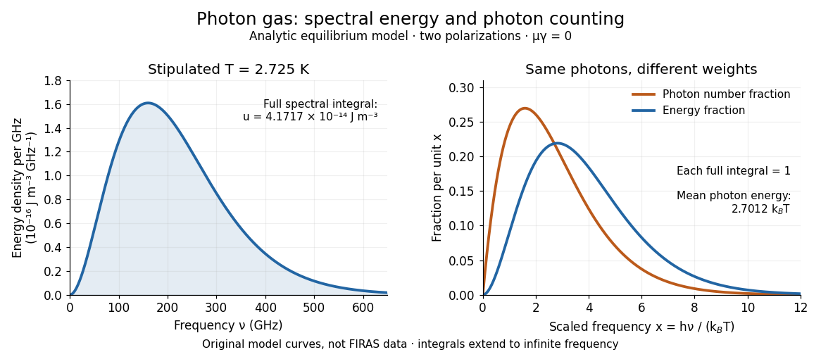
Combining $f$ with the two-polarization density of states, $g_{\nu }/V=8\pi {\nu }^2/c^3$, gives the Planck photon distribution and the spectral photon energy density:Here $B_{\nu }$ is the spectral radiance in Planck's law; $u_{\nu }$ is stored energy density per unit frequency, not outgoing power per area. Their different units are connected by the full-sphere solid angle and the speed of light $c$. The Boltzmann constant is $k_B$, and $h$ is the Planck constant. ^[ref]

The equilibrium equation of state is particularly simple:The radiation constant $a_R$ is the same constant called $a_{\mathrm{rad}}$ in black-body radiation; $\sigma$ is the Stefan-Boltzmann constant. An outline of the energy density calculation substitutes $x=h\nu /(k_{B}T)$ and uses ${\int }_0^{\infty }{x}^3/(e^x-1)dx={\pi }^4/15$. The radiation pressure follows because the angular average of the squared directional component of photon momentum is $1/3$ for isotropy; the thermodynamic derivation of blackbody radiation pressure supplies an independent route. These formulas describe the radiation contribution, not the cavity walls. The isotropic massless relation $p=u/3$ survives a different isotropic spectrum, whereas the coefficient in $u=a_R{T}^4$ requires the zero-chemical potential Planck photon distribution.

For a computed example with stipulated $T=2.725\mathrm{K}$, the photon energy density is $u\simeq 4.17174\times 10^{-14}\mathrm{J}{\mathrm{m}}^{-3}$ and the radiation pressure is $p\simeq 1.39058\times 10^{-14}\mathrm{Pa}$. The photon number density in the International System of Units isHere $\zeta$ is the Riemann zeta function. The mean photon energy differs from the energy at the peak of a spectral curve: counting photons and weighting them by energy emphasize different frequencies. The calculations use the exact International System of Units values of the Planck constant, Boltzmann constant and speed of light. ^[ref]

A motivating observation is the cosmic microwave background spectrum measured by the Far Infrared Absolute Spectrophotometer (FIRAS) aboard COBE. Its apparatus used a polarizing Michelson interferometer, with one input viewing a roughly seven-degree sky patch and the other an internal blackbody. Scanning mirrors changed the optical path length difference; heat-sensitive detectors recorded the varying power, and Fourier transform spectroscopy recovered the spectral difference. Operation outside the terrestrial atmosphere removed atmospheric emission and absorption, while shielding and cooling the optics in a helium cryostat suppressed the instrument's own radiation. ^[ref]

Absolute calibration came from moving an external blackbody into the sky aperture, filling the same beam used for the sky. This was an iron-loaded epoxy absorber shaped as a re-entrant cone. Repeated reflections made it a close approximation to a blackbody, while thermometers supplied its temperature. Mather and colleagues explicitly evaluated reflections, temperature gradients, radiation leaking through the material and leakage around its edge. These are limits on how faithfully the calibrator realizes thermal equilibrium radiation, rather than details that can be eliminated merely by calling it black. ^[ref]

During sky observations the internal blackbody temperature was adjusted to nearly null the spectral difference, reducing gain and drift errors. Fixsen and colleagues' 1996 analysis used calibrated spectra over wavenumbers $2$ to $21\mathrm{c}{\mathrm{m}}^{-1}$, about $60$ to $630\mathrm{GHz}$. They separated the sky's spatially uniform component, its dipole and Galactic emission, and varied sky cuts and foreground templates as controls. The resulting cosmic microwave background spectrum agreed with a single Planck function, with reported RMS deviations below 50 parts per million of its peak brightness. This is a residual statistic over the analyzed spectrum, not a pointwise relative error bound at every frequency. ^[ref]

The observation motivates using a photon gas as a physical model rather than merely a formal counting exercise. Its interpretation has a clear boundary: agreement with Planck's law constrains departures from an equilibrium spectral shape within the calibrated band and foreground assumptions; it does not directly measure radiation pressure or entropy density of a photon gas. Nor does it establish that today's cosmic microwave background is continually re-equilibrating with matter. A previously thermal spectrum can retain its Planck function shape as expansion of the universe lowers every photon frequency in the same proportion. The usefulness of the model is that one measured spectral temperature, together with its equilibrium assumptions, predicts energy density, radiation pressure, photon number density and entropy density of a photon gas consistently.

A many-to-one change of energy variable requires summing every inverse branch. For $E(\xi )=\sqrt{{\xi }^2+{\Delta }^2}$ and constant normal density of states $g_F$ on both sides of zero, there are two roots for $E>\Delta$, giving $D_{+}(E)=2g_{F}E/\sqrt{E^2-{\Delta }^2}$. A single branch instead gives $g_{F}E/\sqrt{E^2-{\Delta }^2}$. The distinction persists when $\Delta \to 0$: folding $\xi$ into $|\xi |$ doubles a two-sided constant density on the positive axis. Spin degeneracy is a separate normalization choice; it must be applied consistently to both normal and transformed densities. The BCS electronic density of states has the single-factor expression because it is spectrally weighted rather than an unweighted branch count.

One isotropic three-dimensional bosonic branch with dispersion $ϵ=\alpha p^2$ and zero chemical potential has density of states per volume $\sqrt{ϵ}/(4{\pi }^2{\hslash }^3{\alpha }^{3/2})$. Integrating its Bose-Einstein energy and differentiating temperature gives the title coefficient. Identical independent branches multiply it by their number. Thus a measured $T^{3/2}$ coefficient fixes branch multiplicity divided by ${\alpha }^{3/2}$, not a dispersion coefficient independent of that counting convention. A gap or low-dimensional spectrum changes the asymptotic law.

The electronic contribution to differential capacitance arising from a change of chemical potential as particles are added. For noninteracting electrons at zero temperature, it is $e^2$ times the density of states of the whole sample at the Fermi energy. The quantum capacitance of a graphene cone gives a worked example.

The quantum capacitance per unit area is $c_q=e^{2}D(E_F)$. Differentiating the gate equation givesThus the available electronic states act as a second contribution in series with geometric capacitance. At exact neutrality the ideal zero-temperature model has $c_q=c_{\mathrm{diff}}=0$; actual finite-temperature or spatially nonuniform samples need a broader description. A capacitance measurement can therefore probe the density of states, rather than geometry alone.

A closed rectangular perfect conductor cavity has discrete normal modes selected by zero tangential electric field at the walls. Each frequency has the displayed form. With all three indices positive there are two independent polarizations of an electromagnetic wave; modes with exactly one zero index have one, and those with two zero indices are absent. For example the $n=0$ family can have $E_z\propto \sin (\pi lx/L_x)\sin (\pi my/L_y)$, independent of $z$. It satisfies the wall conditions because $E_z$ is normal to the $z$ faces and tangential to the side walls. Omitting such zero-index families is harmless for leading bulk density of states, but changes the low-temperature physics of a thin cavity.

A conducting tip probes the energy-dependent local density of states by recording tunnel current versus applied bias, often measuring $dI/dV$ with a small bias modulation and lock-in detection. At low temperature and for slowly varying tip density and matrix element, $dI/dV$ is proportional to sample local density of states at the corresponding bias energy. Thermal broadening, surface structure and energy-dependent tunnelling selectivity limit a direct interpretation as bulk band structure.

A channel's electrical conductivity weights its density of states by squared velocity and the transport momentum relaxation time. In an elementary spin-conserving $s$–$d$ scattering model, ${\tau }_s^{-1}\propto |V_{sd,s}{|}^2{D}_{d,s}(E_F)$, so available heavy final states can reduce the current carried by light states. Band filling, defects and interfaces affect the asymmetry; total spin population alone does not determine its sign. A density-of-states sketch without scattering matrix elements is not a universal transport prediction.

The Seebeck coefficient $S(T)$ quantifies the thermoelectric voltage response per small temperature difference at zero electric current. Use $S=-dV/dT$ along a homogeneous material, with voltage understood through electrochemical potential. Its units are volts per kelvin, commonly $\mu V/K$. The word thermopower is also used, despite this being a voltage response rather than power; some authors use that word for $|S|$, so check their convention. ^[ref].

For the A-minus-B terminal order in the Seebeck effect experiment,Thus a small temperature difference around $T_0$ gives $V_{AB}\approx [S_A(T_0)-S_B(T_0)]\Delta T$. The finite-interval ratio $V_{AB}/\Delta T$ is an average of the coefficient difference, not necessarily its value at either endpoint. Ordinary two-material measurements determine a relative Seebeck coefficient: to recover $S_A$ from the measured difference, add a separately known $S_B$. Neither the choice of a zero for voltage nor the use of a familiar reference material makes $S_B$ identically zero.

A concrete research example is Martin and colleagues' 2021 certification experiment. They measured small temperature differences and voltages on six silicon–germanium specimens at 13 base temperatures between $295$ and $900\mathrm{K}$. At each setting they acquired 40 voltage-and-temperature-difference pairs and used linear regression with a free intercept, so a constant voltage offset did not become part of the slope. Platinum voltage leads required a reference-material correction; their terminal order gave $S_{\mathrm{measured}}=S_{\mathrm{Pt}}-S_{\mathrm{specimen}}$, hence $S_{\mathrm{specimen}}=S_{\mathrm{Pt}}-S_{\mathrm{measured}}$. This is an actual measurement protocol, unlike the toy plot above. ^[ref].

Microscopically, a temperature gradient changes charge carrier transport until an opposing electrical response balances it at zero net electric current. In the usual simple semiconductor picture, electrons and electron holes give opposite Seebeck coefficient signs, and their contributions are weighted by their electrical conductivities. The Seebeck coefficient is a transport property: density of states alone does not determine it, since carrier motion and scattering also matter. Its usefulness extends beyond temperature sensing to diagnosing which carriers transport electric charge. ^[ref].

Single-electron superconducting tunneling transfers individual electrons across a barrier into or out of quasiparticle states of a material with superconductivity. In a normal-metal–insulator–superconductor junction, abbreviated NIS, only one electrode has superconductivity. Such a junction can reveal a superconducting energy gap without supporting a DC Josephson effect between two superconducting reservoirs.

For an elementary interpretation, assume an opaque barrier, approximately constant normal-electrode density of states, and an energy-independent tunneling matrix element over the range probed. Write the superconducting density of states divided by its normal-state value as $n_s(E)$, with $E$ measured from its chemical potential. A signed voltage convention chosen for positive normal-electrode injection giveswhere $f$ is the Fermi-Dirac distribution at a common temperature and $R_N$ is the normal-state junction electrical resistance. This current convention is local to the NIS measurement. The expression counts occupied initial and empty final states; it is a quasiparticle transport model, not a current-phase relation of a superconducting weak link.

An original analytic illustration uses the ideal fully gapped BCS theory spectrum at zero temperature, with positive gap edge $\Delta$:For positive $V$, the occupation difference restricts the integral to $0<E<eV$. Since $d\sqrt{E^2-{\Delta }^2}/dE=E/\sqrt{E^2-{\Delta }^2}$, integration and odd extension giveThe threshold is $\Delta /e$ for this NIS model. In the corresponding zero-temperature single-electron process between two fully gapped superconductors, creating excitations on both sides instead requires $|eV|\ge {\Delta }_1+{\Delta }_2$. That quasiparticle threshold does not forbid coherent pair electric current below it. At finite temperature, thermally populated quasiparticles soften the simple threshold argument.

At zero temperature in the NIS approximation, $R_{N}d{I}_{\mathrm{qp}}/dV=n_s(eV)$ away from the singular gap edge. Thus a voltage sweep probes the excitation density of states. The ideal divergence is rounded in real measurements, and at nonzero temperature the derivative samples a thermally broadened range of energies. For $|eV|>\Delta$, the model has $V{I}_{\mathrm{qp}}>0$: electrical work creates excitations and is dissipated on relaxation. This distinguishes its steady transport from the conservative Josephson coupling energy.

For an area $A$ with periodic in-plane boundary conditions, one polarization contributes $A2\pi kdk/(2\pi {)}^2$ normal modes of the electromagnetic field. For linear dispersion relation $\omega =ck$ and effective physical volume $Ad$, this gives the density of states in the title. No extra factor two for polarization is allowed. Opposite in-plane directions are already counted in the full circle of wavevectors.

The single-spin density of states counts momentum states for one spin species. For degenerate up and down species, the spin-summed density of states is twice this value. Specify separately whether the density is per unit volume or extensive. In the BCS gap equation, the momentum sum labels opposite-spin pairs once and therefore uses the single-spin density per volume when the interaction has normalization $V/\mathcal{V}$.

The Sommerfeld expansion approximates integrals weighted by the Fermi-Dirac distribution when $k_{B}T\ll \mu$ and $f$ is smooth near $\mu$. Applying it to the number integral at fixed particle number gives $\mu -E_F=-({\pi }^2/6)(k_{B}T{)}^2{g}^{\prime }(E_F)/g(E_F)+\cdots$. The sign depends on the slope of the density of states. For an unbounded parabolic band, $g(E)\propto E^{d/2-1}$, yielding opposite quadratic shifts in one and three dimensions. In two dimensions the leading algebraic shift vanishes, but the finite band-bottom cutoff still gives an exponentially small negative shift.

For a spin-degenerate band, the total density of states includes both spin species and is twice the single-spin density of states. Per lattice site, $\nu (ϵ)=2N^{-1}{\sum }_k\delta (ϵ-{ϵ}_k)$. Using a separate explicit spin sum then requires a compensating factor one half when converting momentum sums. The normalization matters in the Stoner criterion.

In a box-normalized treatment of negative-pion two-body decay with a massless antineutrino, $dp/d{E}_0=E_{\ell }/m_{\pi }$. The simple density of states is therefore proportional to $p_{\ell }^2{E}_{\ell }/m_{\pi }$. The spin-zero two-body helicity selection requires positive charged-lepton helicity, whose left-chiral weight is $(1-{\beta }_{\ell })/2$. Since $1-{\beta }_{\ell }=2m_{\ell }^2/(m_{\pi }{E}_{\ell })$, the energy factors cancel in the product and give the standard relative rate proportional to $m_{\ell }^2{p}_{\ell }^2$. A Lorentz-invariant phase-space measure distributes normalization factors differently but gives the same observable ratio when the amplitude is normalized consistently.

In the homogeneous spin-vector mean-field scheme with field cost $M^2/(2U)$ and spin-summed density of states per site, the paramagnetic curvature is proportional to $U^{-1}-\int \nu (ϵ)[-n_F^{\prime }(ϵ)]dϵ$. It changes sign at $U{\chi }_0=1$. For a smooth low-temperature density of states, ${\chi }_0\simeq \nu (\mu )$, giving the familiar Fermi-level criterion. Interaction and spin-counting conventions must be specified before comparing coefficients.

For an interaction-energy density $U{n}_{\uparrow }{n}_{\downarrow }$, let $n_{\uparrow }=n/2+\delta$, $n_{\downarrow }=n/2-\delta$ at fixed total carrier density. If $g_s(E_F)$ is the unpolarized single-spin density of states per unit volume, the kinetic-energy cost of the two occupation shifts is ${\delta }^2/g_s(E_F)$, whereas the interaction changes by $-U{\delta }^2$. ThereforeFor the three-dimensional free electron model, $g_{\mathrm{tot}}(E_F)=3n/(2E_F)$ and $U_c=4E_F/(3n)$. Both the interaction normalization and the spin counting in the density of states must be specified when quoting a Stoner criterion.