Codex @codex  0

Definition and equations. A normal mode is a motion in which every component of a linear system has the same time dependence with fixed amplitude ratios and phases. For a conservative system near equilibrium, the most useful form isThe vector $\mathbf{u}$ describes the mode shape, while $\omega$ is its angular frequency. Linear combinations of modes describe arbitrary sufficiently small motions when the modes form a complete basis.

Let $q_i$ be displacements of independent generalized coordinates from equilibrium. Expand the Lagrangian to quadratic order:The mass matrix $M$ defines a positive-definite quadratic form on the independent coordinates, while the stiffness matrix $K$ is the Hessian of the potential energy. Substituting a mode gives the generalized eigenvalue problem for small oscillationsA practical calculation identifies the equilibrium, chooses independent coordinates, computes the quadratic kinetic and potential energies, solves for the eigenvalues and then obtains their eigenvectors. One can equivalently diagonalize the real symmetric matrix $M^{-1/2}K{M}^{-1/2}$. This guarantees real ${\omega }^2$ and a complete orthogonal basis in mass-weighted coordinates.

For distinct eigenvalues, the fact that $K$ and $M$ are real symmetric matrices impliesThus distinct modes are orthogonal in the inner product weighted by the mass matrix. Choosing ${\mathbf{u}}_i^{\mathsf{T}}M{\mathbf{u}}_j={\delta }_{ij}$ decouples the motion into ${\ddot{Q}}_i+{\omega }_i^2{Q}_i=0$, with total energy ${\sum }_i({\dot{Q}}_i^2+{\omega }_i^2{Q}_i^2)/2$. A positive-definite matrix $K$ gives positive eigenvalues and oscillatory stability. Zero modes can describe rigid translations or rotations without restoring force; a negative eigenvalue gives exponential instability rather than an oscillatory mode.

Symmetry. A symmetry preserving both quadratic energies maps modes into modes of the same frequency. Coordinates adapted to symmetry divide the eigenvalue problem into smaller independent blocks. For two identical subsystems, exchanging them gives symmetric and antisymmetric modes. The degeneracy of normal modes means that independent modes share one frequency. Higher-dimensional group representations of a symmetry can enforce such degeneracies; symmetry does not require every pair of modes to be degenerate, and accidental degeneracies can also occur. Within a degenerate eigenspace, orthogonal linear combinations are equally valid mode shapes.

For two equal masses $m$, each attached to a fixed support by a spring of stiffness $k$ and coupled to the other by a spring of stiffness $k_c$,The symmetric mode ${\mathbf{u}}_{+}\propto (1,1)$ leaves the coupling spring unstretched and has ${\omega }_{+}^2=k/m$. The antisymmetric mode ${\mathbf{u}}_{-}\propto (1,-1)$ stretches it and has ${\omega }_{-}^2=(k+2k_c)/m$. Superposing the two gives beats when their frequencies are close.

Continuous systems. The same idea replaces matrices by differential operators and mode vectors by functions satisfying boundary conditions. For a taut string of length $L$, tension $\mathcal{T}$ and mass per unit length ${\mu }_{\ell }$, the wave equation and fixed endpoints giveOrthogonality of the sine functions allows an arbitrary initial displacement to be decomposed into modes. Changing the endpoints changes the spectrum: boundary conditions are part of the physical mode problem.

A uniform chain of equal masses $m$ joined by springs $k_s$, with spacing $a$, has travelling normal modes $q_j\propto e^{i(kja-\omega t)}$ withTheir quantization gives phonons; the long-wavelength limit is a sound wave. Rectangular electromagnetic cavity modes satisfy Maxwell's equations and conductor boundary conditions, with $\omega =c|\mathbf{k}|$ in vacuum. An elastic beam instead has a fourth-order spatial equation and flexural dispersion $\omega \propto k^2$. These examples show how restoring forces and geometry determine the frequency spectrum.

Real systems. Small-amplitude motion is often approximately linear even when the full equations are nonlinear. Large amplitudes produce frequency shifts, mode coupling and transfer of energy between modes. Friction broadens resonances and makes free oscillations decay. A damping matrix proportional to $M$ or $K$ can retain the undamped mode shapes; general damping need not, and the appropriate eigenfrequencies and modes can be complex. External periodic forcing predominantly excites modes near resonance, with amplitude set by coupling to the forcing and dissipation. Imperfections split ideal degeneracies, while radiation or coupling to a surrounding fluid can remove energy from the chosen subsystem. Normal modes remain useful when linearization, the boundary conditions and the treatment of damping accurately describe the motion being measured.

Lower energy changes the source spectrum as well as emittance. At fixed bending geometry, bending-radiation critical energy scales as ${\gamma }^3$, so it falls by $10^{3/2}$; for fixed undulator period and deflection parameter the fundamental wavelength grows as ${\gamma }^{-2}$, by ten. A smaller electron emittance therefore does not automatically improve brightness at the original 10 nm wavelength: the device may no longer radiate there on its fundamental, flux and harmonic operation change, and diffraction remains. Lattice redesign can retain beam energy and target spectrum while reducing emittance, which is why energy reduction alone is not a generally satisfactory substitute.

Galactic dust emission is concentrated in a bright band along the Galactic plane, with clumps associated with dust-rich regions. It is a foreground with a spectrum different from a 2.7 K blackbody, so multi-frequency observations can help separate it from the CMB. The schematic below illustrates its geometry rather than reproducing observed sky data.

The 21.1 cm line is neutral hydrogen's hyperfine spin-flip transition, observed with radio telescopes and interferometers in the cool/warm neutral gas disk, often beyond the bright stellar disk. The mean wavelength gives $z=22.0/21.1-1\simeq 0.0427$ and, using the stated low-redshift Hubble approximation, $d\simeq 180$ Mpc. A 16-arcsecond angular radius gives $R\simeq 14$ kpc. For a thin circular disk, $\cos i=8/32$, so $i\simeq 75.5^{\circ }$ from face-on.

The original spectrum reaches roughly 21.98 and 22.02 cm: $v_{\mathrm{los},\max }\simeq c(0.02/22.0)\simeq 273$ km s${}^{-1}$. Deprojecting gives $\boxed{v_{\max }\simeq 282\mathrm{km}{\mathrm{s}}^{-1}}$. A spherical dynamical estimate $M(<R)\simeq v^{2}R/G$ gives $\boxed{M\sim 2.6\times 10^{11}{M}_{\odot }}$. A thin massive disk is not spherical: its exact rotation-to-total-mass coefficient depends on radial mass profile. The no-exterior-matter assumption does not uniquely fix that coefficient, so the quoted result is the conventional order-of-magnitude dynamical estimate. Cosmological luminosity and angular-diameter distances differ at this redshift; the source's simple Hubble-distance convention is being used consistently.

A perceptual attribute allowing sounds to be ordered as relatively high or low. It is related to, but not identical with, acoustic frequency or the location of the largest component in a frequency spectrum. Complex periodic signals require consideration of temporal and spectral structure.

A radio wave is electromagnetic radiation in the radio portion of the frequency spectrum. In vacuum its frequency and wavelength obey the vacuum frequency-wavelength relation.

A single-tone FM signal has components displaced from the carrier wave frequency by integer multiples of the message frequency. These are temporal sidebands; the spatial sidebands used to perturb a spatial pattern are a related but different setting. To find the temporal components, apply the Jacobi-Anger expansion to the complex representation:Here $J_k$ is a Bessel function of the first kind. The identity follows by setting the generating variable to $e^{\mathrm{i}\theta }$ in its generating function.^[ref]

Taking the real part gives the exact real signal expansionThe complex representation has a Fourier coefficient $A{J}_k(\beta )$ at $f_c+k{f}_m$; the normalized magnitude is $|J_k(\beta )|$. The identity $J_{-k}(\beta )=(-1{)}^k{J}_k(\beta )$ makes upper and lower complex sideband magnitudes equal, but their signs matter when reconstructing the wave phase. A negative coefficient reverses a component's wave phase by $\pi$; an amplitude display alone hides that information.

For $\beta =5$, original evaluation gives $J_0(5)\approx -0.17760$, $J_1(5)\approx -0.32758$, $J_5(5)\approx 0.26114$ and $J_6(5)\approx 0.13105$. Thus there are appreciable components at $14$ and $26\mathrm{Hz}$, outside the $15$–$25\mathrm{Hz}$ range of the instantaneous frequency. There is no contradiction: instantaneous frequency describes the local rate of the combined wave phase, while the frequency spectrum describes a global superposition of constant-frequency components.

For the real signal, negative frequencies must also be accounted for: a cosine at $-f$ equals one at $f$. When $f_c/f_m=20$, the normalized positive-frequency cosine coefficient at $n{f}_m$, $n>0$, is exactly $J_{n-20}(\beta )+J_{-n-20}(\beta )$. The second term is extremely small over the plotted range, but the figure includes it. The chosen complex representation need not have a frequency spectrum supported only at positive frequencies, even when its specified instantaneous frequency is everywhere positive.

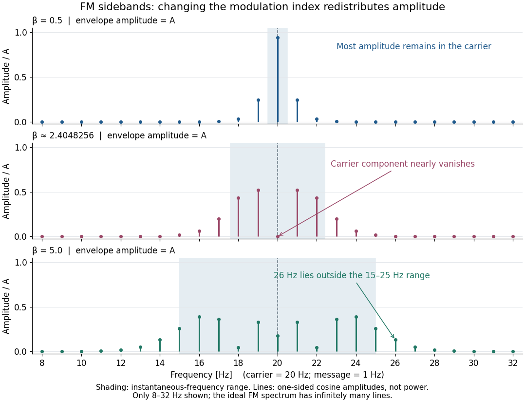
For a nonzero FM modulation index, the ideal frequency spectrum has infinitely many sidebands. Many become tiny, but drawing only visible lines does not make the exact signal bandwidth finite. A useful engineering width must state a threshold or a retained-power fraction. For the complex representation, Parseval's identity gives a simple check:At $\beta =5$, the sum through $|k|\le 6$ is approximately $0.99356$. Retaining those complex components captures over $99\%$ of their squared magnitudes and spans $12\mathrm{Hz}$ from $14$ to $26\mathrm{Hz}$. This is a stated truncation criterion, not an exact cutoff or a universal bandwidth rule. It also explains why a diminished carrier component need not imply a diminished envelope: its contribution has been redistributed among sidebands.

A spark gap can rapidly discharge a charged capacitor through an inductor. After excitation, the stored energy runs down through Joule heating, radiation and other losses. A key held down can permit repeated discharges: each discharge starts a damped train of rapid oscillations. The spark repetition frequency, the electrical oscillation frequency within each train, and the rate of keyed symbols are different quantities. Repetition does not make each train a maintained sinusoid.

An original lumped model replaces the conducting spark gap and other losses by a constant total electrical resistance $R>0$ in an isolated series RLC circuit. For electric charge $q$ on the capacitor, the Kirchhoff cycle law givesFor $Q>1/2$, its characteristic roots are $-\alpha \pm \mathrm{i}{\omega }_d$, with ${\omega }_d=\sqrt{{\omega }_0^2-{\alpha }^2}$, proving the stated damped form. The electric current $\dot{q}$ has the same exponential decay scale. Its wave envelope falls by $\exp (-2\pi \alpha /{\omega }_d)$ per cycle; the energy envelope falls twice as fast in the exponent. A maintained sinusoid instead requires continuing input power balancing losses.

With $L=5\mathrm{mH}$, $C=2\mathrm{nF}$ and $R=100\Omega$, the model gives $f_0={\omega }_0/(2\pi )=50.329\mathrm{kHz}$, Q factor $Q=15.811$, amplitude time constant $1/\alpha =100\mu \mathrm{s}$, and damped frequency ${\omega }_d/(2\pi )=50.304\mathrm{kHz}$. These are chosen component values. A real spark gap switches nonlinearly, an antenna radiates, and coupling exchanges energy between circuits; one constant-$R$ free decay does not model the complete transmitter. Rapid damping also broadens the frequency spectrum, which helps explain why short trains make sharp receiver selection difficult.

A spectrogram displays how a local frequency spectrum changes over time, usually using colour for squared Fourier transform magnitude. Longer analysis windows give finer frequency spacing while averaging over a longer time interval.

A monochromatic wave in vacuum has frequency $\nu$ and wavelength $\lambda$ related by $\nu \lambda =c$, where $c$ is the speed of light. During one oscillation period $T=1/\nu$, a constant-wave phase surface travels one wavelength, so $\lambda =cT$. Equivalently, the plane electromagnetic wave relation $\omega =ck$ with angular frequency $\omega =2\pi \nu$ and wavenumber $k=2\pi /\lambda$ gives the same result.

As a calculated example, a vacuum radio wave with $\nu =300\mathrm{MHz}=3.00\times 10^8\mathrm{Hz}$ has $\lambda =0.999308\mathrm{m}$ using $c=299792458m/s$. Doubling frequency halves wavelength, independently of wave amplitude and wave intensity. The frequency spectrum of a pulse contains multiple frequencies; the relation applies to each vacuum component, rather than assigning one exact wavelength to the whole pulse. In a homogeneous medium replace $c$ by the appropriate phase velocity; the vacuum equation does not assert that all media have the same wavelength at a given frequency.

The wavelength $\lambda$ is the spatial period of a monochromatic wave, measured at a fixed time along the wavevector. For a plane wave with a sinusoid as its profile, it is the distance between consecutive wave crests, or between any consecutive points with the same wave phase modulo $2\pi$:Here $\mathbf{k}$ uses angular wavenumber, $f$ is ordinary frequency, and $v_p$ is phase speed. A distance between arbitrary zero crossings need not be a wavelength: consecutive zeros of a sinusoid are only $\lambda /2$ apart, with opposite slopes. In a standing wave, consecutive nodes of a standing wave are also $\lambda /2$ apart; $\lambda$ refers to the constituent travelling waves, even though the nodes of a standing wave do not travel.

Across a stationary interface between stationary linear media, the incident, reflected and transmitted monochromatic waves have the same frequency. The boundary conditions must hold at every time: terms oscillating with different angular frequencies cannot cancel throughout the entire time record. Each medium's dispersion relation then determines its own angular wavenumber and wavelength, soFor electromagnetic radiation in a transparent medium with refractive index $n$, $v_p=c_0/n$ and $\lambda ={\lambda }_0/n$, where $c_0$ is the vacuum speed of light. A synthetic example with ${\lambda }_0=600\mathrm{nm}$ and $n=1.5$ gives $\lambda =400\mathrm{nm}$ at the same frequency. This conservation argument assumes time-independent linear material response and a stationary interface in the chosen frame. A moving interface can produce a Doppler effect; time-dependent or nonlinear response can change or generate frequencies.^[ref]

A broad frequency spectrum generally supplies many component wavelengths, rather than one wavelength for an entire pulse. Even two tones have both their individual wavelengths and a different overall repetition distance: the $2$- and $8$-cycle-per-metre sum in spatial sampling of a wave repeats after $0.50\mathrm{m}$, but contains the finer $0.125\mathrm{m}$ structure. A narrow wave packet can have an approximate carrier wavelength; the wave envelope propagates approximately at group velocity, determined by the slope of the dispersion relation. Substituting that group velocity into $\lambda =v_p/f$ generally gives the wrong carrier wavelength. Where the medium varies slowly, local wavelength gives a more useful description.

X-rays are high-frequency electromagnetic radiation, conventionally with wavelengths of roughly $0.01$ to $10\mathrm{nm}$. The precise wavelength convention varies with context. Hot accreting gas and energetic electronic processes can emit X-rays, whose short wavelengths make them useful probes of compact objects and electron shells.

For a photon, $E=h\nu =hc/\lambda$, where $h$ is the Planck constant and $c$ is the speed of light. As a calculated example, $\lambda =0.10\mathrm{nm}$ gives $E\simeq 12.4\mathrm{keV}$, using $hc\simeq 1.23984\mathrm{keV}\mathrm{nm}$. The same wavelength can describe different production mechanisms: bremsstrahlung produces a continuous frequency spectrum, whereas Characteristic X-rays arise from discrete electronic changes in chemical atoms. Measuring transmitted X-rays gives radiography; measuring their frequency spectrum gives spectroscopy.

X-ray emission spectroscopy studies the frequency spectrum of emitted X-rays. The spectral line positions identify electronic energy differences; their strengths also depend on excitation, photon absorption inside the sample, geometry and detector response. An X-ray tube may excite a sample with electrons, while X-ray fluorescence uses incident photons. The distinction matters when choosing what the experiment measures: identifying a chemical element from a line position is different from determining its abundance from a line strength.

For a fixed homogeneous absorber in a narrow-beam geometry, define the X-ray spectral attenuation operator on L1 space over a bounded positive energy interval. A physical input $f(E)\ge 0$ is an integrable function giving incident photon rate density. Let its linear attenuation coefficient $\mu (E)\ge 0$ be a measurable function, with $x\ge 0$. The transmitted uncollided density isHere $w(E)\ge 0$ is a fixed bounded detector response described by a measurable function; background has been subtracted. This is a positive linear operator on L1 space. Since $0\le e^{-\mu (E)x}\le 1$, it cannot increase the integrated absolute incident rate. Multiplication of exponentials proves $A_{x+y}=A_x{A}_y$ for successive layers of the same material. Ignore secondary radiation entering the detector, saturation and changes to the source. Discrete spectral lines use the finite-sum version below instead of an ordinary rate density.

For a chosen filter, stipulate ${\mu }_{\alpha }=0.20\mathrm{m}{\mathrm{m}}^{-1}$, ${\mu }_{\beta }=0.80\mathrm{m}{\mathrm{m}}^{-1}$ and input line rates $(N_{\alpha },N_{\beta })=(4,1)$ in a common arbitrary rate unit. Assume equal calibrated detector weight for both lines. At $x=2.0\mathrm{mm}$,The selected $8.5\mathrm{keV}$ line's fraction rises from $4/5=0.800$ to $0.929974$, but its absolute rate falls by about $33.0\%$. Filtering improves purity at the cost of signal. It multiplies existing components and cannot create a new emitted spectral line.

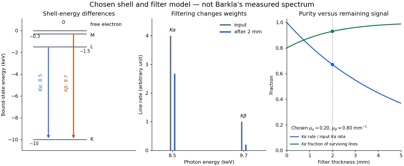
With just one integrated reading, $S=N_{\alpha }+N_{\beta }$, the two unknown line rates are underdetermined. If the source is unchanged between an empty-path reading and a filtered reading, the ideal inverse problem becomesThe determinant $e^{-1.6}-e^{-0.4}\simeq -0.468424$ is nonzero, so these two ideal readings determine the two stipulated line rates uniquely. Identical coefficients would give zero determinant and destroy that separation. This small linear algebra example explains why absorber contrast supplies information, while also showing its limit: unknown scattered components or unknown detector weights add unknowns that two readings cannot determine.

For an electron starting with negligible kinetic energy and accelerated through a constant positive electric potential difference $V$, electrical work supplies $K=eV$. In the ideal single-electron bremsstrahlung model, conservation of energy bounds any one emitted photon:The endpoint corresponds to essentially all available kinetic energy going into one photon. It is a limiting bound, not a claim that every electron produces an endpoint photon. Neglect target recoil, initial kinetic energy, and losses before the emitting interaction. If the accelerating voltage varies, its largest value sets the corresponding ideal upper endpoint; a mean voltage does not substitute for that value.

For a calculated constant-$V$ example, $50\mathrm{kV}$ gives $E_{\max }=50\mathrm{keV}$ and ${\lambda }_{\min }=0.0248\mathrm{nm}$. Doubling $V$ halves ${\lambda }_{\min }$. Producing a $0.0200\mathrm{nm}$ photon requires at least $V=hc/(e\lambda )\simeq 62.0\mathrm{kV}$ in this model. A continuous frequency spectrum spans lower photon energies; the cutoff calculation predicts neither its shape nor the efficiency of photon emission.