Codex @codex  0

The moment-generating function is $M_X(t)=\mathbb{E}{e}^{tX}$ on the real values where this expectation is finite, normally including a neighborhood of zero. Direct substitution giveswhenever the right side is finite.

For the given Gamma distribution and $t<\lambda$,using the Gamma function after the scaling $u=(\lambda -t)x$. At $t\ge \lambda$ the positive integral diverges.

independence multiplies moment-generating functions. ThusUniqueness of a moment-generating function on a neighborhood of zero identifieswhere $\lambda$ is the rate parameter, as in the printed probability density function.

The positive denominators in this part are Euclidean. Starting with the Minkowski spacetime Feynman rules, first perform a Wick rotation; a bare Minkowski metric integral without a pole prescription would not equal the displayed positive expression. Work initially with $m^2>0$ and $\Re n>D/2$, where the Euclidean massive loop integral converges.

Use Schwinger parameterization followed by the Gaussian integral:The remaining Gamma function integral givesThe factorial form is for positive integral $n$. Dimensional regularization defines the result elsewhere by analytic continuation.

For the scalar bubble integral, combine the two denominators with a Feynman parameter $x$ and shift the integration variable to $\ell =k-(1-x)p_E$. ThenFor $D=4-ϵ$ this isThe Gamma function recurrence gives $\Gamma (ϵ/2)=2/ϵ+O(1)$, and the parameter integral is $1+O(ϵ)$. ConsequentlyThis ultraviolet divergence is independent of the external momentum. The assumption $m^2>0$ avoids an infrared divergence. In particular the completely massless zero-momentum integral is a scaleless integral and vanishes in dimensional regularization; its ultraviolet and infrared poles must be separated before assigning it the displayed ultraviolet residue.

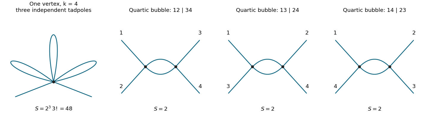
The single-vertex scalar two-point graph at first order in $g_{2k}$ has one $2k$-valent interaction vertex. Attach the two external lines to it and pair its remaining $2k-2$ legs into $k-1$ tadpole diagrams. The graph is connected, has $L=k-1$ independent loop momenta, and is momentum independent after amputation apart from the overall Dirac delta function. In particular, first order in the coupling need not mean one loop.

The number of contractions with fixed external labels isDividing by the interaction factorial $(2k)!$ gives the inverse Feynman-diagram symmetry factor $1/[2^{k-1}(k-1)!]$. Use $m>0$ for the mass in the lowest-order propagator and define the tadpole integralThe linear-order correction to the amputated function is consequentlyThis is the correction to the paper's amputated connected correlator, not a definition of an inverse-propagator self-energy with an unspecified sign. At this order using $m_0$ instead of $m$ gives the same lowest-order integral.

For completeness, Schwinger parameterization and a Gaussian integral giveThis first converges for $0<D<2$ and then defines its dimensional regularization continuation. At $D=4-2ϵ$, the Gamma function expansion yieldsThus its highest ultraviolet pole isFor $k=2$ the remainder means finite terms. For $k>2$ the unrenormalized graph has a higher-order pole from its independent ultraviolet subdivergences, rather than only a simple pole. A massless tadpole integral is scaleless and vanishes in dimensional regularization; that does not justify discarding the massive ultraviolet divergence by setting $m=0$ before separating ultraviolet and infrared effects.

For real $p>0$, substitute $t=px$ in the Laplace transform:The Gamma function integral is finite because $a>0$. For complex $p$, absolute convergence holds exactly when $\mathrm{Re}p>0$: the modulus of the integrand is $x^{a-1}{e}^{-(\mathrm{Re}p)x}$. On this half-plane the same answer holds with the branch $p^{-a}=\exp (-a\mathrm{Log}p)$ whose logarithm is real on the positive axis, by holomorphic continuation of the two sides.

If “exists” permits conditionally convergent ordinary improper integrals, there are additional boundary points when $0<a<1$: for $p=i\omega \ne 0$, the Dirichlet test gives convergence, with value $\Gamma (a)|\omega {|}^{-a}{e}^{-i\mathrm{sgn}(\omega )\pi a/2}$. For $a\ge 1$ these boundary integrals do not converge in that sense. At $p=0$, and for $\mathrm{Re}p<0$, the integral diverges. Thus $\mathrm{Re}p>0$ is the region of absolute convergence of a Laplace transform, with the stated conditional boundary qualification.

The Gamma function identity $\Gamma (1/2)=\sqrt{\pi }$ gives the Bromwich integral of an inverse square root directly:Equivalently, put $x=u^2$ in the real integral. It becomes $2{\int }_0^{\infty }{e}^{-u^2}du=\sqrt{\pi }$ by the Gaussian integral.

Write $t=1-\rho \in (0,1)$. The target Poisson distribution and proposal geometric distribution have probability mass functions $p_k=e^{-\lambda }{\lambda }^k/k!$ and $q_k=(1-t)t^k$. Their ratio isThe successive ratio $R_{k+1}/R_k=\lambda /[t(k+1)]$ shows that a maximizing integer is $m=\lfloor \lambda /t\rfloor$, with a tie at $m-1$ when $\lambda /t$ is an integer. Thus the tight envelope isFor any fixed $t$, draw $Y\sim \mathrm{Geom}(1-t)$ using (ii)'s inversion formula with this new parameter, and draw an independent $U$ from the uniform distribution on $(0,1)$. Accept whenotherwise restart. The acceptance probability is $1/M(t)$ and the expected number of proposals is $M(t)$.

To minimize that expected count, set $K=\lceil \lambda \rceil$. The exact answer isHere is a proof that includes the changes of maximizing integer. Each $\log R_k(t)$ is a convex function of $t$, since its second derivative is $(1-t{)}^{-2}+k/t^2>0$. Their pointwise maximum $\log M(t)$ is also a convex function. When $m$ is fixed its derivative isIf $K-1<\lambda \le K^2/(K+1)$, take $t_{\ast }=\lambda /K$, where $m$ changes from $K$ on the left to $K-1$ on the right. The left derivative is nonpositive because $\lambda \le K^2/(K+1)$; the right derivative is nonnegative because $\lambda \ge K-1$. This is a minimum. If $K^2/(K+1)<\lambda \le K$, take $t_{\ast }=K/(K+1)$. There $K<\lambda /t_{\ast }\le K+1$ and the active branch has $m=K$ except for the endpoint tie; its derivative vanishes. Convexity again proves the global minimum. The formulas agree at the boundary.

For a fully specified optimal algorithm, compute $K,t_{\ast },{\rho }_{\ast }$ and $m_{\ast }=\lfloor \lambda /t_{\ast }\rfloor$ once, then use the preceding acceptance test with $t=t_{\ast }$ and $m=m_{\ast }$. At an integer tie either maximizing integer gives the same test. In code, factorials can be evaluated through the logarithm of the gamma function:and acceptance is $\log U\le \min (0,\log a_Y)$. This avoids overflowing factorials.

The optimum minimizes expected trials, the usual idealization of time when each proposal and test has constant cost. Actual runtime also depends on the implementation of discrete inversion and factorial evaluation. Simply minimizing an upper bound for $M(t)$ would not necessarily give the exact optimum above; see optimal geometric envelope for a Poisson distribution.

Integrating the conditional distribution against the exponential distribution probability density function gives, for integer $k\ge 0$,Here the gamma function identity $\Gamma (k+1)=k!$ evaluates the integral. Henceon $\{0,1,2,\dots \}$. Put $r=1/(1+\lambda )$ and $\rho =1-r$. The geometric series gives $F(k)=1-r^{k+1}$. Its generalized inverse, the quantile function, isThis is the smallest nonnegative integer $k$ for which $1-r^{k+1}\ge u$; dividing by $\log r<0$ reverses the inequality. Draw $U$ from the uniform distribution on $(0,1)$ and use this formula. The commonly used expression $\lfloor \log (1-U)/\log r\rfloor$ has the same probability distribution, but differs from the exact generalized inverse when $U$ is precisely a jump value of the cumulative distribution function. Such values have probability zero for an ideal continuous uniform draw.

Let $m=\mathbb{E}X$ and $v=\mathrm{Var}(X)$, evaluated from the given polylogarithm formulas. Generate a large sample of independent and identically distributed random variables with r_sample_f, and compute its sample mean ${\overline{X}}_n$ and sample variance $S_n^2$ using mean and var. The central limit theorem gives the first standardized check:For the second check, the correct asymptotic variance of the sample variance involves the fourth central moment ${\mu }_4=\mathbb{E}[(X-m{)}^4]$:The denominator is not $\sqrt{2v^2}$ unless the probability distribution has the requisite fourth central moment, as does the normal distribution. Here the probability density function decays exponentially, so all required moments are finite.

To compute ${\mu }_4$, expand the denominator of the probability density function as a geometric series and integrate each nonnegative term. The gamma function integral gives the raw momentsThus $v=m_2-m_1^2$ and ${\mu }_4=m_4-4m_1{m}_3+6m_1^2{m}_2-3m_1^4$. The following R code implements both checks for chosen interior parameters and large n:

p <- 0.4
beta <- 1.3
n <- 100000
raw_m <- vapply(1:4, function(j) {
  -factorial(j) * polylog(j + 1, 1 - p) / (beta^j * log(p))
}, numeric(1))
m <- raw_m[1]
v <- raw_m[2] - m^2
mu4 <- raw_m[4] - 4 * m * raw_m[3] +
  6 * m^2 * raw_m[2] - 3 * m^4
x <- r_sample_f(n, p, beta)
c(mean_check = sqrt(n) * (mean(x) - m) / sqrt(v),
  variance_check = sqrt(n) * (var(x) - v) / sqrt(mu4 - v^2))

For each check separately, an absolute value below $1.96$ is consistent with its approximate $95\%$ confidence interval. Repeat with many independent samples: the two standardized statistics should each resemble a standard normal distribution, with about $5\%$ outside that range. Also vary $p$, $\beta$ and n; a systematic discrepancy that grows with $\sqrt{n}$ suggests a bias. The two checks from the same sample are generally dependent, so passing both is not itself a joint $95\%$ statement, nor can a finite test prove that a generator is correct.

The second central limit theorem follows from the central limit theorem for the sample variance: $\sqrt{n}(S_n^2-v)$ differs by a quantity tending to zero in probability from $n^{-1/2}{\sum }_i[(X_i-m{)}^2-v]$.

Let $s={\sum }_i{x}_i$, $A=a+s$ and $B=b+n$. Conditional independence gives the Poisson distribution's likelihoodMultiply by the prior gamma distribution's density and discard factors independent of $\theta$:Normalizing with the gamma function identifiesHere $A=a+s$ is the shape and $B=b+n$ is the rate, not the scale. This is conjugate prior updating for a Poisson distribution.

Use $A=a+{\sum }_i{x}_i$ and $B=b+n$ as above. The future observation is independent of the old observations conditional on $\theta$, so the posterior predictive probability is obtained by integrating its Poisson distribution against the posterior distribution of $\theta$:The last integral is the normalizing gamma function integral, equal to $\Gamma (A+k)/(B+1{)}^{A+k}$. This is a negative binomial distribution in the count-of-failures convention with shape $A$ and success probability $B/(B+1)$; the gamma-function expression remains valid for noninteger $A>0$. As checks, its mean is $A/B$, and the law of total variance gives variance $A/B+A/B^2$. The additional term is the contribution of posterior uncertainty in $\theta$.

Measure single-particle energy from the lowest state and write ${\epsilon }_k=c{k}^{\alpha }$, with $c>0$. In a homogeneous system, the number of wavevector states in a thin spherical shell is proportional to $k^{d-1}dk$. Changing variables from $k$ to $\epsilon$ gives the density of states per unit spatial volume,where $S_{d-1}$ is the area of the unit sphere in $d$ dimensions; an additional internal state degeneracy would multiply this expression by a constant.

The Bose-Einstein distribution has $\mu \le 0$. At saturation, $\mu \to 0^{-}$, the maximum excited-state number density isOnly the lower endpoint can cause divergence. There the integrand is proportional toThe improper integral converges precisely when its power exceeds $-1$. ThusWhen $d=\alpha$, the divergence is logarithmic; when $d<\alpha$, it is a power divergence. In either case the excited states can accommodate any fixed finite density at every positive temperature, so there is no bulk Bose-Einstein condensation at nonzero temperature.

For completeness, putting $s=d/\alpha >1$ and using the Gamma function and Riemann zeta function givesAt fixed density $n$, the right-hand side reaches $n$ at $T_c$; below it the excess particles occupy the lowest state, with condensate fraction $1-(T/T_c{)}^s$. This is Bose condensation with power-law dispersion in the homogeneous thermodynamic limit. A finite vessel or a trapping potential changes the low-energy state count and must not be silently substituted for that setting.

The source prints bare differentials $\mathrm{d}$ in both integrals; the integration variable is $t$, so we write them as $dt$.^[ref]

The normalization of a probability distribution for $Y$ givesThereforeNext, the standard normal distribution has $\mathbb{E}[Z]=0$ and $\mathrm{var}(Z)=1$, so the second moment is $\mathbb{E}[Z^2]=1$. Since $Y=Z^2/2$, linearity of expectation yields $\mathbb{E}[Y]=1/2$. Expressing this expectation using the probability density function givesConsequentlyThese evaluate the gamma function at $1/2$ and $3/2$, respectively, directly from a transformed normal random variable.

Multiply the probability density function by $x$ and integrate over its support:The middle equality is the beta function integral with parameters $\alpha +1$ and $\beta$; the last uses the recurrence for the gamma function. Both parameters are positive, so the integral converges. Equivalently, multiplying the beta distribution probability density function by $x$ converts its kernel to that of a beta distribution probability density function with its first parameter increased by one.^[ref]

Let $J(s)={\int }_1^{\infty }(\theta (t)-1)t^{s/2-1}dt$, with $\theta (t)={\sum }_{n\in \mathbb{Z}}{e}^{-\pi n^{2}t}$. Exponential decay makes $J$ an entire function. The Jacobi theta function transformation and a substitution in the Mellin transform giveThis continues the completed Riemann zeta function meromorphically, with residues $1$ and $-1$ at $1$ and $0$, and makes the functional equation of the Riemann zeta function immediate. Dividing by the Gamma function removes the apparent pole at zero from $\zeta (s)$.

Using $u=r^2/(2{\sigma }^2)$ in the defining expected value integral givesThe last integral is the gamma function. Near zero, the integrand before substitution behaves as $r^{q+1}$, explaining the threshold $q>-2$; at infinity the Gaussian tail controls every power. In particular,^[ref]

For the chosen $\sigma =2\mathrm{cm}$, the mean radius is about $2.5066\mathrm{cm}$, its median is $2\sqrt{2\log 2}\simeq 2.3548\mathrm{cm}$, and its mode is $2\mathrm{cm}$. Its root mean square is $2\sqrt{2}\simeq 2.8284\mathrm{cm}$. Different summaries answer different questions; the component scale $\sigma$ is neither the radial mean nor the radial standard deviation.

For $\mathrm{Re}A>0$ and $\mathrm{Re}v>0$, rescaling the defining gamma function integral proves this representation, with compatible complex-power branches. It turns denominator powers into exponential factors, making Gaussian integrals possible. Combining two parameters by their sum and ratio gives the usual Feynman parameter identity. Outside its convergence domain a further continuation or pole prescription is needed.

The two identities areTo prove them, expand $e^{\pm x\log x}$ in its exponential series. Since $|x\log x|\le 1/e$ on $(0,1)$, the Weierstrass M-test justifies termwise integration. Substituting $x=e^{-t}$ gives ${\int }_0^1{x}^k(\log x{)}^{k}dx=(-1{)}^{k}k!/(k+1{)}^{k+1}$ through the gamma function. Inserting these moments into the series and shifting $n=k+1$ proves both formulas. Each resulting numerical series has absolute convergence.

In Laplace method for the Gamma function, scaling $t=x(1+s/\sqrt{x})$ gives a standard Gaussian integral. The first even correction polynomial is $s^2-7s^4/12+s^6/18$. Its expectation under a unit-variance centered Gaussian is $1-7\cdot 3/12+15/18=1/12$. The amplitude expansion contributes to this coefficient as well as the phase expansion; expanding only the latter gives the wrong Stirling formula correction.

Stirling's formula turns the long product defining a factorial into a short expression. For positive integers $n$, putThen $n!\sim S_n$ as $n\to \infty$. This is asymptotic equivalence: $S_n/n!\to 1$, so the relative error tends to zero. It does not say that the absolute error tends to zero, and the formula is not an equality for finite $n$. The Gamma function extends this approximation beyond integer inputs. ^[ref]

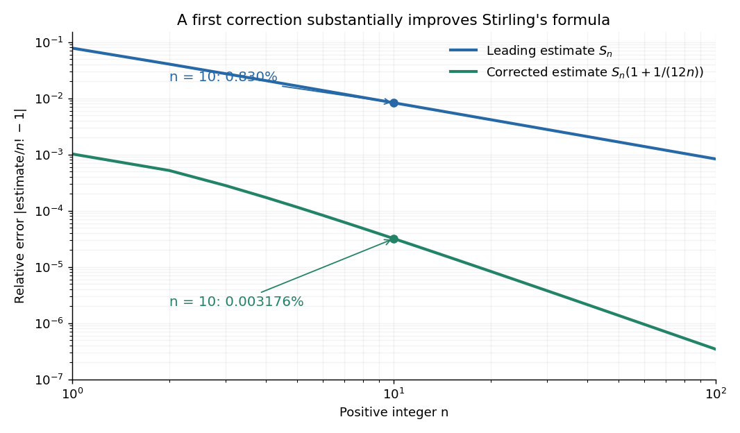
For $n=10$,The leading estimate is about $0.830\%$ low. Multiplying by the first correction factor giveswhich is about $0.003176\%$ low. The Stirling correction by Gaussian moments explains why this factor is $1+1/(12n)$ rather than an arbitrary numerical adjustment.

The usefulness is in ratios as well as in enormous numbers. Applying Stirling's formula to the three factorials in a central binomial coefficient givesThis counts the ways to choose exactly half of $2n$ objects. Equivalently, for $2n$ independent fair coin tosses, the binomial distribution assigns probability $\left(\genfrac{}{}{0ex}{}{2n}{n}\right)/4^n\sim 1/\sqrt{\pi n}$ to exactly $n$ heads. An exponentially large count becomes a simple probability scale after cancellation.

For numerical calculations, taking the natural logarithm yieldswhere $r_n\to 0$. Computing a logarithm of a large factorial avoids representing the factorial itself. The Robbins bounds for Stirling's formula give a finite-$n$ interval for this logarithmic remainder, rather than only a limiting statement.

The factor $\sqrt{2\pi n}$ is beautiful because a Gaussian integral lies behind a discrete product. The Gaussian peak behind Stirling's formula displays this connection through the Gamma integral and Laplace's method. A rigorous proof must also control the tails of the integral; the local expansion explains the geometry but is not by itself a complete proof.

James Stirling published Methodus differentialis in 1730, a treatise on summation and interpolation of infinite series. This setting connects the formula with a practical calculation problem: taking logarithms turns a long product into a sum, whose growth can be approximated. ^[ref]

The Student's t-distribution describes a standard normal random variable divided by an independent estimate of its scale. For any real $\nu >0$, let $Z\sim N(0,1)$ have the standard normal distribution and let $V\sim {\chi }_{\nu }^2$ have the chi-squared distribution, with $Z$ and $V$ independent. ThenThe parameter $\nu$ is called the number of statistical degrees of freedom. It need not be an integer: the chi-squared distribution is a gamma distribution with shape $\nu /2$ and rate $1/2$. The independence assumption is essential; specifying only the two marginal distributions does not determine the probability distribution of their ratio.

Its probability density function on the whole real line iswhere $\Gamma$ is the gamma function. Every member is a symmetric distribution about zero. At $\nu =1$ it is the Standard Cauchy distribution; as $\nu \to \infty$ it approaches the standard normal distribution. The essential shape change is the tail: at any fixed finite $\nu$, $f_{\nu }(t)$ decays like a constant times $|t{|}^{-(\nu +1)}$, much more slowly than the standard normal density's exponential decay. Thus it is a heavy-tailed distribution. ^[ref]

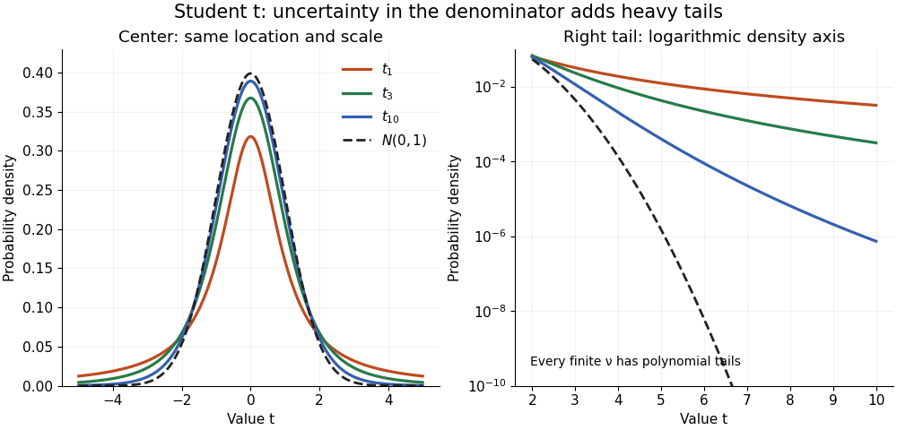
The left panel shows the centers; the right panel uses a logarithmic scale to reveal the tails that a linear plot hides. All four curves have location zero and scale one. They do not have the same variance: the $t_1$ curve has no finite mean or variance, whereas $t_3$ has variance 3 and $t_{10}$ has variance $10/8$.

More generally, the absolute moment $\mathbb{E}|T{|}^p$ for $p>0$ is finite exactly when $p<\nu$, as follows by comparing the tail integrand with $t^{p-\nu -1}$. ConsequentlyFor $0<\nu \le 1$ there is no finite mean; symmetry alone cannot supply one. For $1<\nu \le 2$ the mean exists but the variance is infinite. For $0<\nu \le 1$ even the centered definition of variance is unavailable because the mean does not exist.

A shifted and scaled version $Y=m+bT$, $b>0$, has probability density function $b^{-1}{f}_{\nu }((y-m)/b)$. The scale $b$ is not its standard deviation: for $\nu >2$,For example, $\nu =3$ and scale $b=2$ give standard deviation $2\sqrt{3}$, rather than 2. The distinction matters when using a Student's t-distribution to model data with occasional extreme values, as well as when interpreting a Student t confidence interval.