Codex @codex  0

A function is discontinuous at a point in its domain of a function when it fails the epsilon-delta definition of continuity there. Two basic failures are an incorrect assigned value and unequal one-sided limits. They demand different repairs.

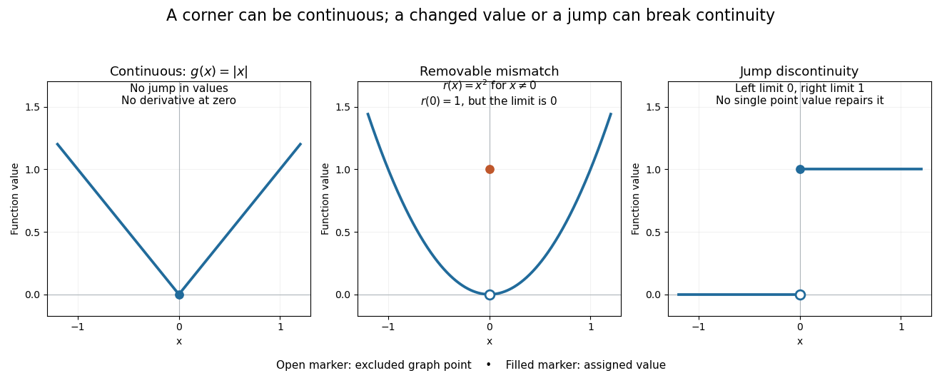
For a removable discontinuity, considerThe limit at zero is $0$, but $r(0)=1$. Replacing that one value by $0$ gives the continuous square function. The sequence $x_n=1/n$ makes the mismatch visible: $r(x_n)=1/n^2\to 0\ne r(0)$. A removable discontinuity can also describe an expression with a missing value, in which case the question is whether a continuous extension to the missing input exists.

For a jump discontinuity, take $j(x)=0$ for $x<0$ and $j(x)=1$ for $x\ge 0$. The left and right one-sided limits at zero are $0$ and $1$. No assignment to $j(0)$ can equal both, so changing only the point value cannot make the function continuous there. Contrast both examples with the corner of $|x|$: that function is continuous at zero even though its derivative is absent.

The finite volume method follows the amount of a conserved quantity inside each control volume. Its unknowns are cell averages, rather than values at isolated points: a cell's width times its stored average approximates that cell's total. A numerical flux transfers an amount across a face. Using one shared transfer for both neighboring cells makes the loss from one exactly the gain of the other, as explained in shared face flux cancellation.^[ref]

For a one-dimensional scalar conservation law without sources, let $u_t+{\partial }_{x}f(u)=0$, with conservation law flux $f$. Fix cells $I_j=[x_{j-1/2},x_{j+1/2}]$ of widths $h_j>0$. Define the exact cell average and its numerical approximation byThe integral balance over one cell and one time interval of length $k>0$ isFor a smooth solution this follows by integration of the differential equation; with jump discontinuities, it expresses the conservation law in integral form, using appropriate face traces when they exist. Replacing each time-averaged face conservation law flux by a numerical flux givesThus the finite volume method implements a balance directly, without needing a pointwise derivative at a jump. The tube balance in Riemann Problems and Jupyter Solutions by David I. Ketcheson, Randall J. LeVeque, and Mauricio J. del Razo (Advection, §Conservation of mass) motivates this construction from conservation of mass.

This is useful for shock waves: their speed is constrained by the Rankine-Hugoniot condition, itself an integral balance. A nonconservative approximation can give a visibly plausible jump with the wrong speed. Conservation is one requirement; a nonlinear scalar conservation law also needs the correct entropy solution, and the chosen numerical flux and update need their own stability and accuracy analysis.^[ref] The original periodic upwind finite volume advection example isolates the shared-transfer mechanism in a problem with a known translated solution.

A Fourier series describes a periodic function through sines and cosines whose frequencies are integer multiples of one base frequency. These Fourier harmonics give a useful alternative to describing the value at every input: each Fourier coefficient measures how much of one oscillating pattern is present. For a real, integrable function of period $2\pi$, the real form isThe cosine formula includes $n=0$; the sine formula uses $n\ge 1$. Thus $a_0/2$ is the mean value over a period, not $a_0$ itself. The symbol $\sim$ associates a function with its Fourier coefficients; an equality requires a specified kind of convergence, such as pointwise convergence. For general period $T>0$, replace $nx$ by $2\pi nt/T$ and the coefficient prefactor by $2/T$. Fourier orthogonality explains why integrating against one mode removes the others. ^[ref].

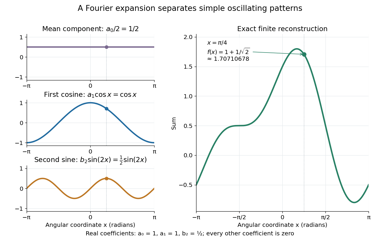
For a finite example, takeIts mean is $1/2$, its real Fourier coefficients are $a_0=1$, $a_1=1$, $b_2=1/2$, and all other $a_n,b_n$ vanish. At $x=\pi /4$, the three contributions add to $1/2+1/\sqrt{2}+1/2=1+1/\sqrt{2}\approx 1.70710678$. The function is already a trigonometric polynomial, so retaining these modes reconstructs it exactly. Here $x$ is an angular coordinate in radians; if it instead represents time, a base angular frequency must supply the corresponding units.

The change of viewpoint is useful because many linear problems act separately on these modes. The second derivative maps $\sin (nx)$ to $-n^2\sin (nx)$ and maps $\cos (nx)$ in the same way. Consequently a differential equation that is complicated for a whole profile can become a simpler calculation for each Fourier harmonic. A linear time-invariant system similarly has a separate response to each complex exponential. Superposition combines the responses when the relevant sums and operations are justified. ^[ref].

The infinite case contains a subtlety absent from the finite example. Under pointwise convergence of a piecewise smooth Fourier series, the value at a jump discontinuity is the average of the two one-sided limits. For a square-integrable function, the complex Fourier series instead converges in the $L^2$ norm: the integrated squared error tends to zero. Neither statement says that the error becomes small everywhere at once. A square wave shows the difference vividly through the Gibbs phenomenon.

A historical source for this connection between profiles and modes is Joseph Fourier's 1822 book Théorie analytique de la chaleur. Chapter III develops expansions in sines and cosines while studying the propagation of heat. The heat equation gives a continuing application of this approach. ^[ref].

For $\beta >0$, periodically extend $\cosh (\beta x)$ and $\sinh (\beta x)$ from $-1<x\le 1$ with period $2$. Their Fourier series areand, away from odd integers,The first identity follows by integration of $\cosh (\beta x)\cos (n\pi x)$ on $[-1,1]$, using the antiderivativeFor the second identity, integration by parts and $d\cosh (\beta x)/dx=\beta \sinh (\beta x)$ show that its sine coefficient is $-n\pi /\beta$ times the first series' cosine coefficient. This avoids assuming that a Fourier series can always be differentiated term by term. The periodic hyperbolic cosine is continuous, so its series converges to it everywhere. The periodic hyperbolic sine has a jump discontinuity at each odd integer: the Dirichlet-Jordan convergence theorem gives the average of its two limiting values, namely zero, there. Both identities hold in the sense of mean-square convergence, which suffices for Parseval's identity.

The Gibbs phenomenon is the persistent overshoot near a jump discontinuity in ordinary truncated Fourier series. For this square wave, retain $M$ nonzero odd modes:As $M$ grows, the first peak approaches the jump while its height tends to approximately $1.17897974$. This is an excess of about $0.17898$ above the upper level $1$, or $8.949\%$ of the jump size $2$. The narrower region does not imply a vanishing maximum error. At the jump itself every $Q_M(0)=0$. These observations are compatible with pointwise convergence and $L^2$ convergence but exclude uniform convergence to the discontinuous square wave. ^[ref].

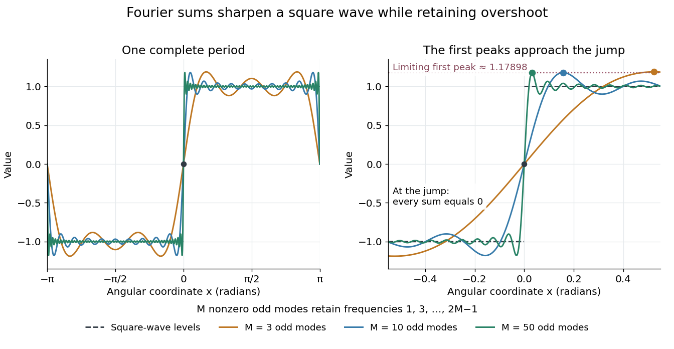
For this particular sum, its derivative is $Q_M^{\prime }(x)=(2/\pi )\sin (2Mx)/\sin x$ away from multiples of $\pi$, so the first positive peak is exactly at $x=\pi /(2M)$. There,This is a midpoint Riemann sum tending to $2\mathrm{Si}(\pi )/\pi$, where $\mathrm{Si}$ is the sine integral. It gives a short explanation of the nonzero limiting excess.

The phenomenon matters whenever a sharp boundary is represented by a limited set of Fourier harmonics: a visible ripple can be a property of the approximation rather than an oscillation in the original profile. Josiah Willard Gibbs reported the phenomenon in his 1899 letter “Fourier's Series” in Nature, volume 59, page 606. This is a documented historical report, without a claim of first discovery. ^[ref].

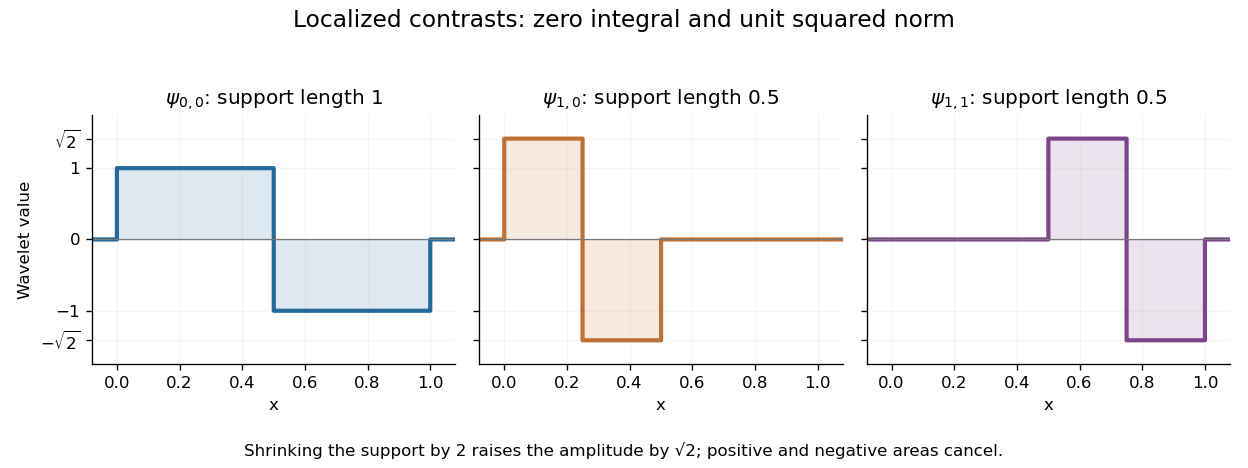
The Haar wavelet is a signed contrast between two adjacent half-intervals:It has compact support, zero integral, and unit L2 norm: $\int \psi =1/2-1/2=0$ and $\int |\psi {|}^2=1$. The zero integral is its one vanishing moment. Its Haar scaling function is $\varphi =1_{[0,1)}$, which records a coarse value rather than a contrast. Endpoint conventions do not alter the L2 inner products.

The normalized copies ${\psi }_{j,k}(x)=2^{j/2}\psi (2^{j}x-k)$ compare the halves of the dyadic interval $[k{2}^{-j},(k+1)2^{-j})$. Narrower copies are taller so that their L2 norms stay one. Thus a coefficient identifies both a location, through $k$, and a scale, through $j$.

For a simple step function $f$ equal to $2$ on $[0,1/2)$ and $6$ on $[1/2,1)$, its coarse coefficient is $⟨f,\varphi ⟩=4$, while its first contrast is $⟨f,\psi ⟩=-2$. Thus $f=4\varphi -2\psi$. The negative coefficient raises the second half and lowers the first. Finer contrasts vanish because $f$ is constant on each half. A jump aligned with this dyadic interval boundary therefore needs only two nonzero coefficients; jumps at other positions can require details at many scales.

Its jump discontinuities make the Haar wavelet particularly transparent for changes between neighbouring regions, while limiting approximation of smooth variation. A Daubechies wavelet uses a more elaborate pattern to obtain additional vanishing moments and, at sufficiently high order, smoother basis functions. The elementary Haar refinement identity has coefficients $h_0=h_1=1/\sqrt{2}$ and explains how the coarse and fine descriptions fit together.

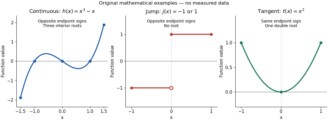
The historical source is Alfred Haar's ^[ref]. Chapter III, beginning on page 361, constructs the constant function and these localized piecewise-constant orthogonal functions. Its original endpoint assignments differ from the half-open convention used here, without changing L2 inner products.

Three explicit functions separate the hypotheses from the conclusion. These are original mathematical illustrations, not measured data.

The polynomial function $h(x)=x^3-x=x(x-1)(x+1)$ is a continuous function on $[-3/2,3/2]$, with $h(-3/2)=-15/8$ and $h(3/2)=15/8$. The intermediate value theorem guarantees at least one zero of a function in the interior, while the polynomial factorization displays three: $-1,0,1$. Thus strict opposite signs do not establish uniqueness.

The everywhere-defined functionhas $j(-1)=-1$ and $j(1)=1$, yet no zero of a function. Its jump discontinuity at zero is exactly where the continuity hypothesis fails. A drawn vertical connector would be misleading: the function graph contains neither the intermediate heights nor a zero of a function at that jump. Even continuity only on the interior is insufficient: setting $q(x)=-1$ for $0\le x<1$ and $q(1)=1$ gives opposite endpoint signs on $[0,1]$ with no zero of a function, because the left one-sided limit at $1$ is not $q(1)$.

The polynomial function $t(x)=x^2$ on $[-1,1]$ is a continuous function, and $t(-1)=t(1)=1$, yet $t(0)=0$. Its root of a polynomial at zero has multiplicity of a root two. The function graph touches its horizontal tangent line there and stays positive on both sides: existence of a zero of a function does not require a sign change. More generally, near a real root of a polynomial $r$, a polynomial factorization $p(x)=(x-r{)}^{2m}u(x)$ with $m\ge 1$ and $u(r)\ne 0$ has the same sign on both sides sufficiently close to $r$, since the continuous function $u$ retains its sign. The intermediate value theorem does not rule out values outside the range between endpoint outputs.^[ref]

Interval bisection solves a target equation $f(x)=t$ by repeatedly halving a closed interval known to contain a solution. It is the bisection method applied to $g(x)=f(x)-t$, so the target becomes a zero of a function. This reduction from an equation to root finding is described in Demanet's notes.^[ref] Here the emphasis is on a continuous strictly increasing function: the target identifies one input, making interval bisection a way to evaluate its inverse function without an explicit inverse formula.

Let $f:[a_0,b_0]\to \mathbb{R}$ be a continuous function, with $a_0<b_0$ and $f(a_0)\le t\le f(b_0)$. The intermediate value theorem guarantees existence; a strictly increasing function also guarantees uniqueness. Check endpoint equality first. Otherwise, for the current root bracket $[a_k,b_k]$, evaluate its midpoint $m_k=(a_k+b_k)/2$. If $f(m_k)<t$, retain $[m_k,b_k]$; if $f(m_k)>t$, retain $[a_k,m_k]$; if $f(m_k)=t$, return that exact solution. These comparisons preserve the target bracket. General bisection method needs continuity and opposite signs of $g$ at the endpoints, without requiring monotonicity or a unique zero of a function; see limitations of bisection.

An original dimensionless polynomial example isHere $f(0)=0<10<30=f(3)$ and the derivative $f^{\prime }(x)=3x^2+1>0$, so there is exactly one solution. In fact $x_{\ast }=2$; knowing this lets us check the computed absolute error independently of the guarantee. The first four halvings give the following exact rational numbers:

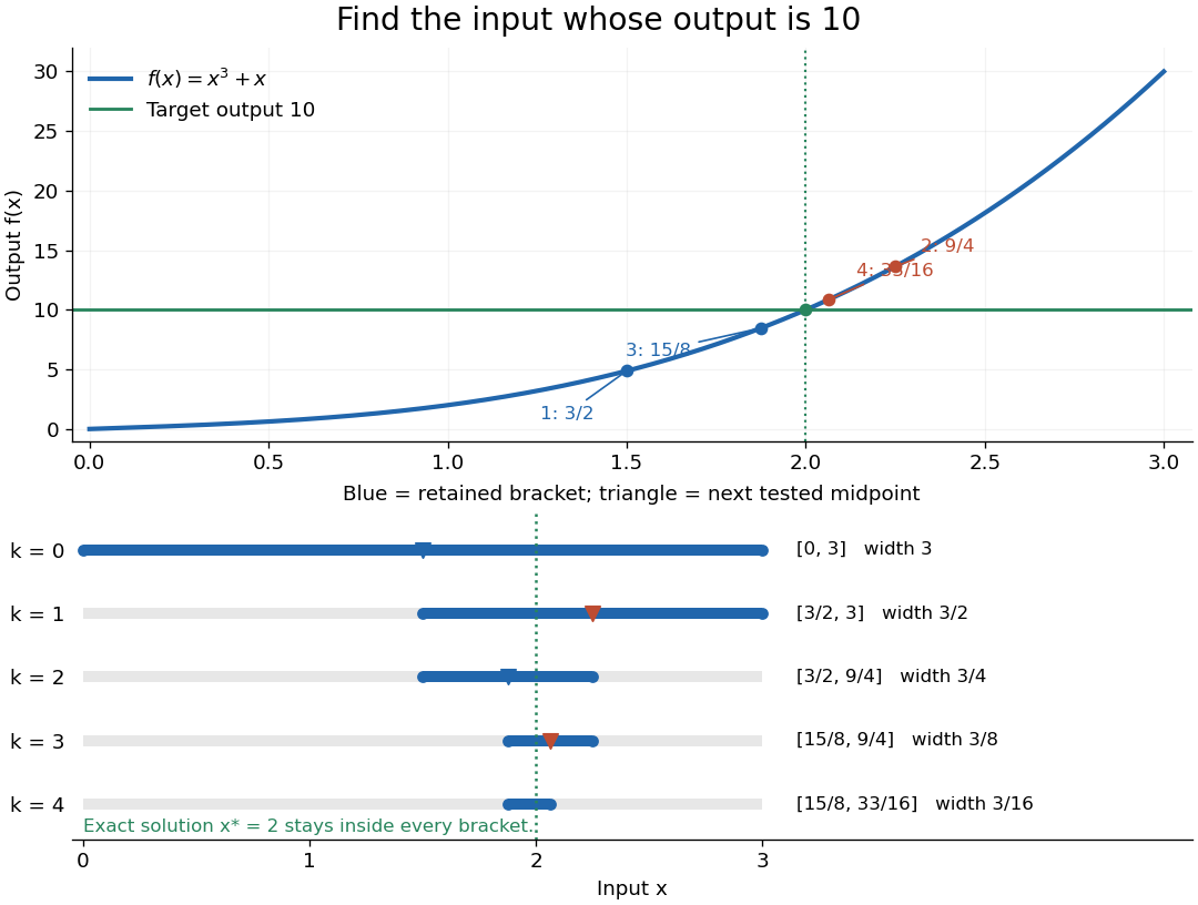
The beauty of interval bisection is that the enclosure itself supplies the certificate: one comparison removes half the possible inputs, regardless of the steepness of the function graph. In exact arithmetic, after $k$ completed halvings without exact termination, the width and the bisection error bound for the new midpoint areThe reported midpoint after update four is $m_4=63/32$, rather than the last tested point $m_3=33/16$. Its certified absolute error is at most $3/32$, and its actual absolute error is $1/32$. For a requested position tolerance $10^{-3}$, the bisection stopping criterion requires eleven halvings: ten give $3/2048>10^{-3}$, while eleven giveThe actual absolute error is $1/4096$. The new midpoint need not be evaluated to obtain this certificate.

The signed output residual is $r=f(m)-t$; the position approximation error is $m-x_{\ast }$. They answer different questions: how close is the output to the target, and how close is the input to the solution? Driscoll and Braun explain why a small residual needs information about the derivative to imply small position error.^[ref] For this particular polynomial, direct factorization givesThus at $m_4=63/32$ the residual is $-13121/32768\approx -0.400421$, despite position absolute error $1/32=0.03125$. If a differentiable function satisfies $0<\ell \le f^{\prime }(x)\le L$ throughout the bracket, the mean value theorem gives the rigorous conversionOur example permits $\ell =1$ and $L=28$ on $[0,3]$. Strict increase alone supplies no positive lower derivative bound: $f(x)=x^3$ is strictly increasing but $f^{\prime }(0)=0$. A small residual alone is therefore not a universal position certificate; even the target equation $10^{-6}(x-2)=0$ has residual $10^{-6}$ at $x=3$, a full unit from its solution.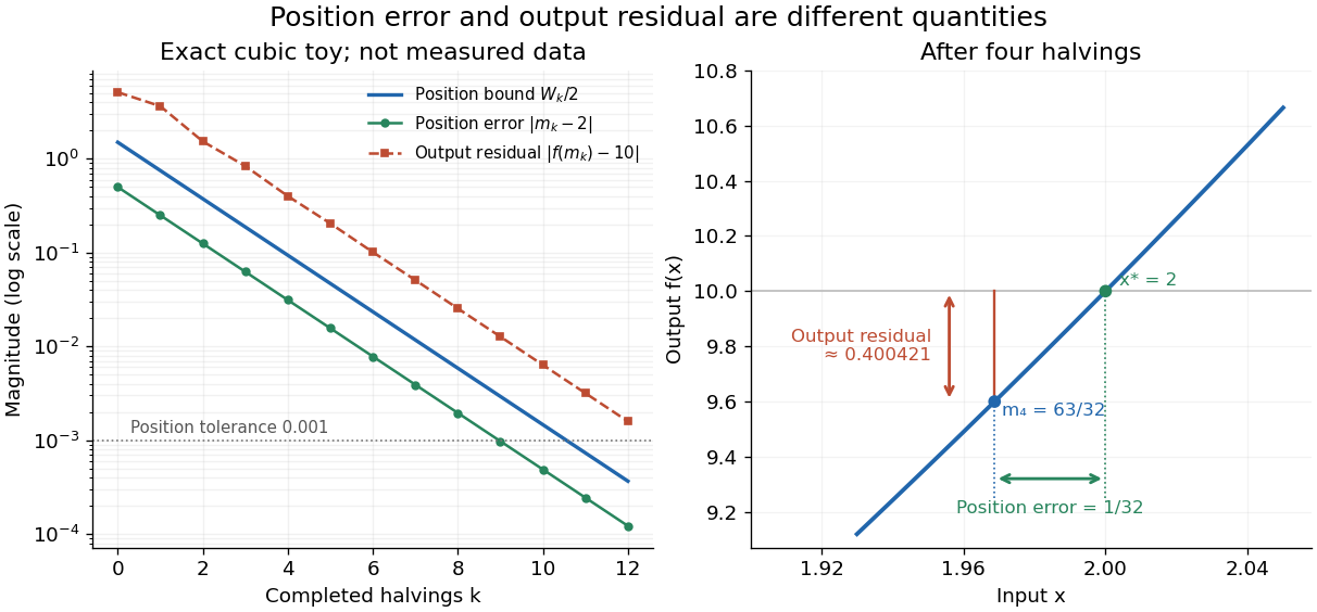

The guarantees require continuity and correct evaluations, not just narrowing endpoints. For the strictly increasing function $h(x)=x$ when $x<0$ and $h(x)=x+1$ when $x\ge 0$, the target $1/2$ lies between $h(-1)$ and $h(1)$ but is never attained: a jump discontinuity defeats the existence argument. With floating-point arithmetic or an approximate evaluation, an incorrect comparison can discard the true solution. A certified interval enclosure of $f(m)$ wholly below or above $t$ certifies the corresponding decision; an enclosure containing $t$ is inconclusive, rather than proof of equality. If rounding makes the midpoint equal an endpoint, report the precision limit; see bisection stopping criterion for the rounded position bound. Both figures are exact mathematical examples, not measured data.

Let $\psi$ be an integrable function with at least one vanishing moment. For a unit jump discontinuity $f(x)=H(x-x_0)$, where $H$ is the Heaviside step function, substitution into the coefficient givesThe signed integral of the whole analyzing function is zero, but the jump discontinuity cuts through its support of a function and usually leaves an unbalanced partial integral. At fixed relative position $\theta$ with nonzero partial integral, the coefficient decays as $\sqrt{a}$, slower than the $a^{q+1/2}$ Taylor remainder bound on a smooth region. “Edges survive” means this relative contrast: the normalized coefficients still tend to zero as $a\to 0$.

For an original exact comparison, use the smooth polynomial $f(x)=x+x^2$ at $b=0$. The Haar wavelet $h$ and the second-difference analyzing function $\eta$ giveThe linear term cancels for $\eta$; it remains for $h$. For the fixed unit jump discontinuity $H(x)$, choose $b=-a/4$ so that $\theta =1/4$ at every scale. Then

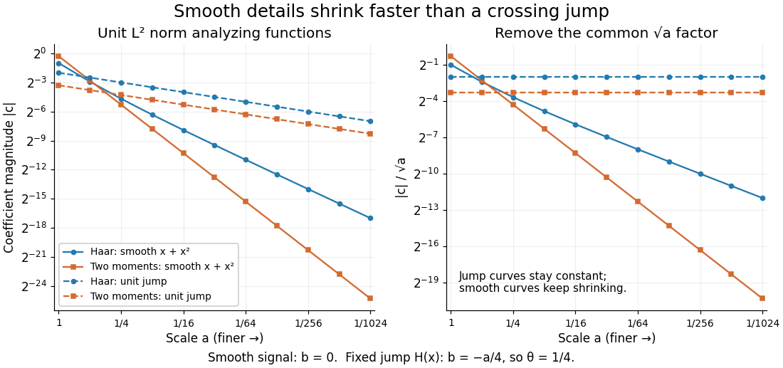
Position matters. If an analyzing function's support of a function lies entirely on one constant side of the jump discontinuity, its coefficient is zero. Even a crossing can cancel: $\eta$ has zero partial integral at $\theta =3/2$. A jump discontinuity on a dyadic interval boundary can likewise escape finer Haar wavelets whose supports do not cross it. These examples describe particular functions and normalizations, not a universal ranking of wavelets for signal processing.

A real-valued function $f:D\to \mathbb{R}$ is a nondecreasing function if every pair $x<y$ in its domain of a function satisfies $f(x)\le f(y)$. Flat intervals are allowed, unlike for a strictly increasing function. For example,is a continuous nondecreasing function, but it repeats its output on each flat interval.

A nondecreasing function can also be discontinuous. The step function $F(x)=0$ for $x<0$ and $F(x)=1$ for $x\ge 0$ has a jump discontinuity at zero without ever decreasing. It is the cumulative distribution function of a random variable that equals zero with probability one; quantile functions handle such jumps through a generalized inverse. Nondecreasing allocation functions permit critical-value payments in single-parameter mechanisms.

For $\beta =1$, $q=(y+x-x^2)/x^2$. On the two sides of the corner-carrying characteristic curve, the partial derivative isAt every point $(x,x^2-x)$ with $x>0$, the two one-sided partial derivatives are $x^{-2}$ and $0$. Therefore $u_y$ does not exist on this curve; its piecewise values have a jump discontinuity of magnitude $x^{-2}$. There are no other interior discontinuities. The values on the outer boundaries are interpreted from within ${\mathcal{D}}_1$.

This is exactly propagation of a derivative jump along a characteristic. Already on $x=1$, the data have slopes $1$ and $0$ on the two sides of $y=0$. The transport equation transports this corner along the characteristic curve from $(1,0)$, which is $y=x^2-x$; it provides no smoothing. This is consistent with Noncharacteristic Cauchy data and does not contradict the smooth-data theorem, whose differentiability hypothesis fails here.

Joseph Fourier's Théorie analytique de la chaleur by Joseph Fourier (1822) makes trigonometric series instruments for solving problems of heat conduction. A prescribed temperature distribution need not be given by one power series: it may describe different heating on different parts of a body. The extract occurs in Chapter III, §233, where the earlier assumption of an odd-power expansion is relaxed. The innovation concerns both representation and what can count as a function in an analytical calculation.^[ref]

Use a separate integration variable $t$ to unpack the printed notation. The proposed Fourier sine series has coefficientsThe integral signs in the extract denote definite integrals over $[0,\pi ]$, not antiderivatives; the author explicitly supplies these bounds in the surrounding sentence. Their absent printed bounds are a notational convention, not permission to choose arbitrary constants of integration.

The key calculation is the orthogonality relationThe product-to-sum formulas prove this by integrating cosines of integer multiples of $t$. If an expansion can be integrated term by term, multiplication by $\sin (mt)$ followed by integration selects exactly one coefficient. This derives the only possible coefficients, but does not by itself prove the expansion converges to the proposed function. That distinction is central to assessing the extract's claim.

For a revealing example take $f(x)=1$ on $0<x<\pi$. Direct integration gives $b_n=2(1-(-1{)}^n)/(\pi n)$, and thereforeEvery term is zero at $0$ and $\pi$, so the series cannot take the value $1$ at those endpoints. Its natural interpretation uses the odd extension followed by periodic extension; the endpoints become jump discontinuities. More generally, for a piecewise continuously differentiable function, the Fourier series converges at an interior jump to the average of the two one-sided limits, irrespective of an individually assigned value there. Changing one value also leaves the integrals unchanged. Consequently the unqualified assertion of representation for every arbitrary function cannot be a modern pointwise theorem. Dirichlet's theorem on Fourier series supplies sufficient conditions and the correct distinction between continuity points and jumps; its 1829 source explicitly addresses the proof problem.^[ref]

The physical payoff is explicit. For a rod scaled to $0<x<\pi$ with zero end temperature, separation of variables in the heat equation producesEach mode solves $u_{\tau }=\kappa u_{xx}$ and the end boundary conditions; the Fourier sine coefficients encode the initial temperature. This rod is an explanatory example, distinct from the stationary rectangular-solid problem opening Joseph Fourier's Chapter III. The factor $e^{-\kappa n^2\tau }$ damps high modes rapidly for positive time. The representation of arbitrary data makes the physical solution possible; the proof of that representation remains a separate task.

The Fourier coefficients satisfy $a_0=a_n=0$ andThus the square wave has Fourier seriesIt equals $f$ away from its jump discontinuities, and converges to $0$ at the jumps. The assigned endpoint values do not affect its Fourier coefficients.

For the Poisson equation, use separation of variables $\varphi ={\sum }_{n\text{ odd}}{b}_n{R}_n(r)\sin (n\theta )$. The radial equation is $r^2{R}_n^{\prime \prime }+r{R}_n^{\prime }-n^2{R}_n=r^2$. Its bounded solution with zero Dirichlet boundary condition at $r=1$ isIndeed the negative power is excluded at the centre, and the boundary fixes the coefficient of $r^n$. No resonance at $n=2$ occurs because only odd modes are forced. ThereforeThis is a Poisson equation on a disk with angular forcing. The series converges uniformly on the closed disk: for $n\ge 3$ each term is bounded by a constant times $n^{-3}$. Its first spatial derivatives also converge uniformly. For instance the radial derivative and $r^{-1}$ times the angular derivative of each term are bounded by constants times $n^{-2}$; the $n=1$ harmonic term is smooth in Cartesian coordinates. It defines a function with zero boundary data and the required weak formulation. Applying the Laplacian to finite partial sums gives the Fourier partial sums of $f$, which converge in $L^2$; passing to the limit against smooth compactly supported test functions verifies the Poisson equation. It holds classically off the jump rays and the centre, where the forcing is locally constant. It cannot be interpreted as a global classical equation with continuous second derivatives for discontinuous forcing. Uniqueness follows from the zero-boundary Dirichlet energy identity for the difference of two solutions.

Finally orthogonality gives ${\int }_0^{2\pi }f(\theta )\sin (n\theta )d\theta =\pi b_n$. The radial integral isUniform convergence of $\varphi$ and boundedness of $f$ justify integration term by term, soThe negative sign also agrees with $\int \varphi \Delta \varphi =-\int |\nabla \varphi {|}^2$. The original PDF's radial denominator is $n^2-4$; the converted TeX's $n^2-1$ is a transcription error.

The precise conclusion is that finite one-sided limits must agree, so a jump discontinuity is impossible. We prove this using explicit kernels and derive every conjugate-series identity used. The distinction from a removable discontinuity is addressed at the end.

Write the Fourier coefficients asTranslation multiplies each coefficient by a unimodular factor and preserves the hypothesis, so place the proposed discontinuity at zero. Suppose the finite limits are $A=f(0^{-})$ and $B=f(0^{+})$. For $0<r<1$, geometric summation gives the Poisson kernel on the circle and the conjugate Poisson kernel on the circle:These series converge uniformly and absolutely for each $r<1$. Therefore they may be integrated term by term against the Lebesgue integrable function $f$. With normalized convolution, $P_r$ has multiplier $r^{|n|}$, while $Q_r$ has multiplier $-i\mathrm{sgn}(n)r^{|n|}$ for $n\ne 0$ and zero at $n=0$. More explicitly, at zero,The assumed vanishing of negative Fourier coefficients thus proves, rather than presupposes, the conjugate relation

We next show that the right-hand side is bounded as $r\uparrow 1$. The kernel $P_r$ is positive and even, and its normalized integral is one by its series. Its mass outside any fixed $(-\delta ,\delta )$ tends to zero; in fact its supremum there is $O_{\delta }(1-r)$. On $(-\delta ,0)$, $f$ is uniformly close to $A$ for sufficiently small $\delta$, and on $(0,\delta )$ it is uniformly close to $B$. Evenness places asymptotically half the mass on each side. The outside contribution tends to zero because $f$ is integrable and the outside kernel tends uniformly to zero. Bounding the inside errors by the one-sided approximation errors givesHence $(Q_r\ast f)(0)$ is bounded by the proved conjugate relation.

On the other hand, oddness of $Q_r$ givesFor $0<\delta <\pi$, differentiating $1-2r\cos t+r^2$ proves the exact identityAlso $Q_r\ge 0$ on $(0,\pi )$ and is uniformly bounded on $[\delta ,\pi ]$ as $r\uparrow 1$. Write $f(-t)-f(t)=A-B+e(t)$ with $e(t)\to 0$ as $t\downarrow 0$. The integral over $[\delta ,\pi ]$ is $O_{\delta }(1)$ by integrability. Given any $\eta >0$, choose $\delta$ so that $|e(t)|\le \eta$ on $(0,\delta )$. Positivity and the preceding identity show that the near-zero error, divided by $\log (1/(1-r))$, has limiting upper bound at most $\eta /\pi$. Letting $\eta \downarrow 0$ provesBoundedness of the numerator makes the left side tend to zero. Therefore $A=B$. This proves one-sided Fourier spectrum excludes jumps, and supplies the required conjugate-sum argument in full.

There is a point-value qualification to the phrase “first kind.” If it means finite unequal one-sided limits, the proof establishes exactly the stated result. If the definition also includes removable discontinuities, the literal statement is false for an arbitrary integrable representative: the function that equals zero everywhere except $f(0)=1$ has every Fourier coefficient zero but a removable discontinuity at zero. Integral hypotheses cannot detect a change at one point. Thus no jump is possible; equal one-sided limits need not equal an arbitrarily assigned point value.

On $(-\pi ,\pi )$ the function is odd, so its mean and all its cosine Fourier coefficients vanish:The assigned endpoint value does not affect these integrals. The product of the two odd functions $x|x|$ and $\sin nx$ is even, hence the sine Fourier coefficients areTwo applications of integration by parts giveThereforeThe periodic extension has a jump discontinuity at every odd multiple of $\pi$: its left and right limits are ${\pi }^2$ and $-{\pi }^2$. Its assigned value at each such point is $-{\pi }^2$. Thus it is odd away from these points, but it is not a globally odd function pointwise. The Fourier series will take the midpoint value zero at these jumps.

The truncated Fourier cosine series gives the better approximation on the closed interval, in the senses of uniform convergence and the asymptotic L2 norm error. To make the comparison precise, let $C_N$ and $S_N$ retain the frequencies $1\le n\le N$, with the constant term also included in $C_N$.

The cosine Fourier coefficients are $O(n^{-2})$. In fact, absolute convergence gives the uniform tail boundFor the Fourier sine series, every Fourier partial sum satisfies $S_N(0)=S_N(\pi )=0$. Thusso there is no uniform convergence to $f$ on the closed interval. Its odd extension has jump discontinuities, producing the Gibbs phenomenon near the endpoints; its Fourier coefficients decrease only like $1/n$.

The advantage persists in the L2 norm, which ignores individual endpoint values. By Parseval's identity and Fourier orthogonality,The nonzero odd cosine coefficients and both parity classes of sine coefficients also give matching lower bounds of these orders by comparison with the corresponding p-series. Hence their L2 norm errors decrease respectively like $N^{-3/2}$ and $N^{-1/2}$. This is a comparison of approximation quality in specified norms, not a claim that one finite sum has smaller error at every individual interior point.

For the Fourier cosine series, integration by parts givesand, for $n\ge 1$,Only odd Fourier harmonics remain, so

For the Fourier sine series, another integration by parts givesConsequentlyAt $x=0$ and $x=\pi$, the Fourier sine series instead has value zero.

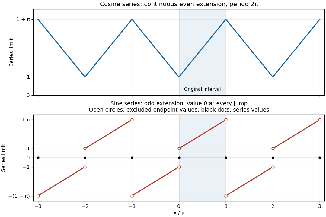
To describe the requested graphs precisely, take $t\in [-\pi ,\pi )$ congruent to $x$ modulo $2\pi$. The Fourier cosine series converges to the continuous triangular periodic extensionIts minima occur at the even multiples of $\pi$, with value $1$, and its maxima at the odd multiples, with value $1+\pi$. The Fourier sine series converges toThe jump discontinuities at even multiples of $\pi$ go from $-1$ to $1$; those at odd multiples go from $1+\pi$ to $-(1+\pi )$. Each jump is assigned its midpoint, zero, by the Fourier series.

Treat the boundary data as $2\pi$-periodic in the angular variable. Denote the outer data by $g(\theta )$, and set $h(\theta )=f(a,\theta )$ for the inner data. Define their mean and nonconstant Fourier coefficients byThe outer data have reflection symmetry, so all their sine Fourier coefficients vanish. Their mean is $1/2$, and their cosine Fourier coefficients are

The angular Fourier harmonics for a single-valued harmonic function in an annulus are $\cos (n\theta )$ and $\sin (n\theta )$, with integer $n\ge 1$. Their radial factors are independent combinations of $r^n$ and $r^{-n}$; the zero angular mode has radial factor $A_0+B_0\log r$. For arbitrary inner data, the sine and cosine modes need independent radial coefficients: forcing them to share one radial factor, as in the product form supplied in the paper, would impose an extra restriction. For either sine or cosine mode, if its outer and inner coefficients are $v$ and $w$, the radial coefficients $\alpha ,\beta$ obeySolving this linear system givesIt is convenient to collect the result into the annular harmonic interpolation factorsThey satisfy $H_n(1)=1$, $H_n(a)=0$, $K_n(1)=0$ and $K_n(a)=1$. The zero mode satisfies $A_0=1/2$ and $B_0=(p_0-1/2)/\log a$. Therefore the required separation of variables solution isAll dependence on $f(a,\theta )$ is given by the displayed integrals. Substituting $r=a$ leaves its Fourier series, and substituting $r=1$ leavesthe Fourier series of the specified outer step. The radial factors satisfy $r^2{R}^{\prime \prime }+r{R}^{\prime }-n^{2}R=0$, so each nonconstant term satisfies Laplace's equation; $1$ and $\log r$ do also. For integrable boundary data the radial factors give exponential decay on every closed subannulus strictly inside $a<r<1$, justifying the necessary termwise partial derivatives there.

There is a qualification at the two outer jump discontinuities. By pointwise convergence of a piecewise smooth Fourier series, the outer series gives $1/2$ at $\theta =\pm \pi /2$, whereas the printed data assign $1$ at those two points. Thus the displayed solution attains the outer data at their continuity points, and has radial limit $1/2$ at the jumps. One may separately assign the boundary value $1$ at the two exceptional points without changing the interior harmonic function, but no continuous extension can match the discontinuous data there. For piecewise smooth inner data, the analogous boundary trace agrees with $h$ at continuity points and with its midpoint at jumps. Some regularity of $h$ is necessary for a classical interpretation; the problem imposes none explicitly.

For period $2$, use the Fourier series conventionThe Fourier coefficients have prefactor $1$ on $[-1,1]$. First, $a_0={\int }_{-1}^1{e}^{x}dx=2\sinh 1$. For $q=n\pi$ the useful antiderivatives areAt the endpoints $\sin (n\pi )=0$ and $\cos (n\pi )=(-1{)}^n$, soConsequently, on $-1<x<1$,The Dirichlet-Jordan convergence theorem justifies equality at every point of continuity of the periodic extension. At odd integers the extension has a jump discontinuity between $e$ and $e^{-1}$, so the series converges to their average $\cosh 1$, regardless of any assigned endpoint value. This is the $\kappa =L=1$ case of the Fourier series of a periodically extended exponential.