Codex @codex 0
Joined 2026-09-21 Message

Incoming links: Linear polarization
When the birefringence separation of optical propagation constants is large compared with the spatial rate of rotation of the optical axes, light with linear polarization in a local eigenpolarization follows the twisting nematic director. Thickness alone is insufficient if birefringence vanishes. Strong field alignment along the propagation direction suppresses the transverse optical anisotropy and hence the quarter-turn polarization rotation.
Beam splitter Created 2026-10-05 Updated 2026-10-14
A beam splitter is an optical instrument that routes an incident beam of light into transmitted and reflected beams. It also combines incident complex amplitudes: two inputs can contribute to the same output. A common geometry has four optical ports, with two chosen as inputs and two as outputs. A beam splitter changes the field; a photodetector supplies a measurement.[ref]
Photon quantum mechanics and beam splitters by Charles H. Holbrow and others. Photon quantum mechanics and beam splitters, §IV, printed p. 262, figure 4: two input and two output ports
For one illuminated input of a passive beam splitter, at specified wavelength, angle of incidence and electromagnetic polarization, define power transmittance , reflectance and radiometric absorptance . In steady operation, with no gain or other source, no net stored energy change, and all escaping light included in the transmitted or reflected collection,This is conservation of energy divided by incident power. If and count only the intended output beams, include a separate scattered or otherwise uncollected fraction : then . Missing output power need not be wave absorption. For an original specified example, , , and give transmitted, reflected and absorbed; these are assumed values, not measurements.
A 50:50 beam splitter specifies equal output powers for one input, not equal complex amplitudes without a relative wave phase. Recombination needs the beam splitter scattering matrix, including its wave phases. A nonpolarizing beam splitter approximately divides both orthogonal linear polarizations in the same power ratio over its specified operating range; a polarizing beam splitter deliberately routes the two differently.
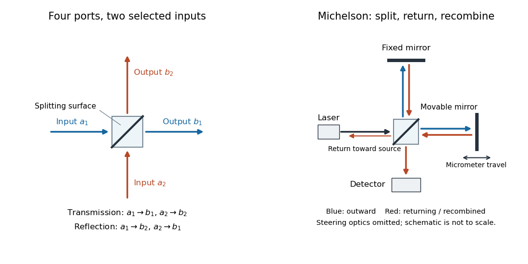
The useful surprise is that the same component divides power with one input and steers power by wave interference with two inputs. In a Michelson interferometer or Mach-Zehnder interferometer, mirror motion changes relative wave phase, turning a small change in optical path length into a measurable change in output power.
Birefringent walk-off 2026-10-14
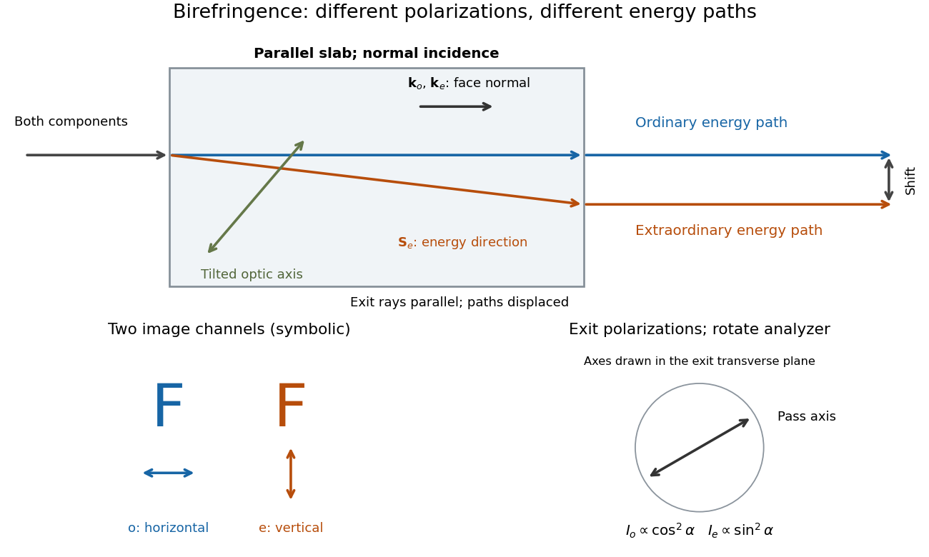
The extraordinary wave's Poynting vector can differ in direction from its wavevector. The latter specifies wave phase propagation, while the former specifies energy flux. This angular separation is walk-off.[ref]
In the lossless, nondispersive model above, take the gradient of to obtain the group velocity, parallel to the Poynting vector. If its angle to the optic axis is , this gives . Consequently the extraordinary wave generally carries energy away from its wavevector direction. An internal wavevector normal to a slab face therefore does not guarantee a normal energy path. Birefringent walk-off vanishes at and ; the latter direction still has unequal refractive indices. This is a useful waveplate geometry: overlapping components can acquire phase retardation without spatial splitting. A thin specimen, insufficient imaging resolution, or excitation of only one linear polarization can also hide a double image, for different reasons.
Brewster solar elevation 2026-10-20
For sunlight reflected from a horizontal flat dielectric interface, incidence angle is measured from the vertical while solar elevation is measured from the horizontal. The Brewster condition therefore gives . Reflected light has its electric field perpendicular to the vertical incidence plane, so its surviving linear polarization is horizontal. This ideal result assumes real refractive indices, negligible absorption, nonmagnetic media and a smooth interface.
Calcite double-image experiment Created 2026-10-14 Updated 2026-10-18
Place a clear calcite specimen on a transparency bearing printed words on an overhead projector. The projected readout is two copies of the lettering. Put a rotatable linear polarizer after the specimen: suitable orientations suppress one copy or the other. These are the actual apparatus and observations in the University of Iowa demonstration.[ref]
Polarization - Calcite & Iceland Spar by University of Iowa, Department of Physics and Astronomy. Demonstration 6H35.15, Equipment and Procedure: crystals, polarizers, printed overhead transparency, two sets of words and selective extinction; final note on natural defects
For a useful control, remove the specimen while keeping the transparency, projector and screen fixed: the doubling should disappear. Replace it, hold it stationary and rotate only the polarizer; complementary brightness changes distinguish two linear polarizations from an accidental duplicate transparency. These are suggested controls, rather than additional reported measurements. Ideally the two copies obey complementary Malus's law curves, and , with angle measured from the exiting ordinary wave's linear polarization. Unequal maxima do not invalidate the test. Finite polarizer extinction, poor focus and specimen defects limit visibility; image separation alone does not determine either refractive index without the specimen geometry.
Circular birefringence 2026-10-18
Circular birefringence means different refractive indices for opposite circular polarizations. In a transparent isotropic medium, their relative wave phase changes rotate the direction of transmitted linear polarization; optical activity gives the solution measurement and convention.
Coherent beam splitter recombination 2026-10-14
Suppose the two input beams share frequency, electromagnetic polarization and overlapping transverse profiles at each output, with stable relative wave phase during the photodetector's averaging interval. For the ideal beam splitter scattering matrix above, expanding the squared complex amplitudes givesThe imaginary part terms describe wave interference. Applying the single-input power split to each input separately and adding the results would discard these terms. Their opposite signs ensure : conservation of energy survives even when one output is dark.
For an original example, let , and . Then and :
| Relative input wave phase | Output power | Output power |
|---|---|---|
At , makes and ; at the dark output swaps. Thus the two inputs can feed all their combined power into one output without gain. At zero relative input wave phase, the splitter's own relative wave phase leaves the contributions in quadrature, so neither output is dark.
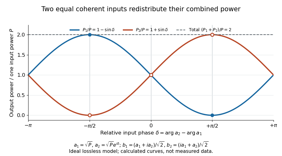
Relative input wave phase redirects the combined power of two coherent beams
. Original ideal-model curves for , and . Output powers are normalized by one input's power ; their sum is always . Markers show the three worked cases. These are calculated curves, not measured data. Details.For fluctuating fields, average the cross term as . It vanishes for mutually uncorrelated inputs, making the independent power-splitting rule valid for the averaged output. Partial first-order optical coherence reduces it. Orthogonal linear polarizations eliminate the cross term in a polarization-insensitive power readout, and spatial mismatch reduces the overlap. Detector averaging can also erase rapid relative wave phase changes. A fixed relation between two inputs can be prepared by splitting one laser beam and recombining the two arms.
An actual teaching protocol in Michelson Interferometer & Precision Wavelength Measurement — Week 1, University of Colorado Boulder, §§4–6, starts with an ideal-model prediction, then builds a Michelson interferometer using a helium-neon laser, a nonpolarizing beam splitter, adjustable mirrors, a micrometer translation stage and a photodetector. Steering mirrors align beam overlap at near and far planes; far-plane interference fringes refine alignment. Moving the arm mirror changes the returning relative wave phase; detector voltage is watched with a live acquisition display or oscilloscope. The guide compares measured arm powers with 50:50 splitting and asks for a revised field model. It tests electromagnetic polarization dependence, optionally changing one arm with a quarter-wave plate, and estimates noise from repeated readings at fixed mirror position. These controls test whether fringe changes reflect coherent recombination rather than splitter imbalance or misalignment. The guide supplies a protocol, not a numerical dataset. Its detector noise, imperfect overlap and electromagnetic polarization mismatch limit displacement inference.[ref]
Additional background subtraction controls follow from the field model: block both arms to record the detector offset and ambient light, then unblock each arm separately to establish its detected power at fixed gain. With both open, scan the mirror and compare extrema after subtracting that background. Keep the detector below saturation and repeat the scan to check drift. A changing signal alone cannot distinguish source optical coherence from motion or changing overlap. For a vacuum round trip, a mirror displacement changes relative wave phase by ; the useful signal is its modulation after detection, not an optical-frequency oscillation that the detector must resolve.
Coherent preparation and incoherent mixing 2026-10-14
Choose the qubit computational basis , also called the basis, and the Hadamard basis , also called the basis. Compare a coherent preparation of with choosing or at random with equal probabilities and discarding that label:These are original ideal preparation models. Their -basis probabilities are both , because their quantum state populations agree. Their -basis probabilities are respectively and . Indeed , whereas . The missing off-diagonal quantum coherence therefore changes a prediction that the common populations cannot determine.
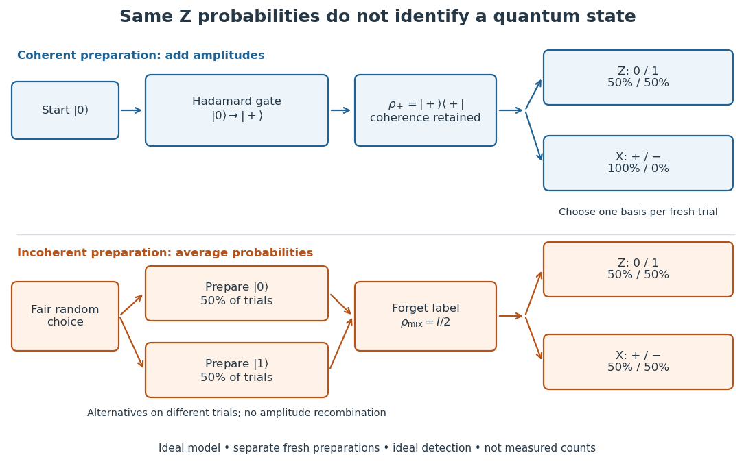
For a relative quantum phase , the coherent family instead hasThe last formula follows by adding or subtracting the two probability amplitudes before taking the squared modulus. At , the state is and the outcomes switch to , while the outcomes remain . In contrast, changes both components by the same global phase and retains the outcomes . In photon polarization, the identification , makes and the two orthogonal diagonal linear polarizations; these labels describe measurement bases, not spatial axes for photon spin.
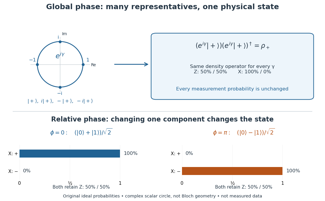
Even perfect statistics in one basis cannot certify a preparation. The above data fit both density matrices. Conversely, distinct preparation histories can yield the same quantum state:The off-diagonal terms cancel in the right-hand ensemble. Every measurement on the qubit alone then has identical probabilities for those two histories. A retained classical label would allow conditioning on different members of the quantum state ensemble; it is extra information beyond the unlabelled density operator.
Double-pass quarter-wave plate 2026-10-18
For a reciprocal ideal quarter-wave plate followed by a mirror at normal incidence, use the same fixed transverse laboratory axes for the forward and returning Jones vectors. If the axes coincide with the plate's fast and slow axes, each pass has Jones matrix up to a common phase factor. A polarization-independent mirror has scalar reflection coefficient , so the returned Jones vector is . The plate acts twice as a half-wave plate, rather than undoing its phase retardation.
For input linear polarization at angle to the fast axis, the returned line is at modulo . At it is perpendicular to the original line. An axis-aligned input instead returns along the same line. General elliptical polarization requires its full input Jones vector; no unique returned state follows from the word “polarized” alone. The propagation direction reverses, so comparing descriptions of circular polarization must also specify the viewing convention.
Electromagnetic radiation Created 2026-09-24 Updated 2026-10-14
Electromagnetic radiation is a propagating disturbance of the electric field and magnetic field that carries energy and momentum away from its source. It can be a sustained electromagnetic wave or a finite wave packet: periodic oscillation is not required. In vacuum the disturbance travels at the speed of light. A receiver responds to fields arriving now from an earlier source event, as expressed by retarded time. This is how electrical activity at one place can deliver energy and information elsewhere without a connecting wire.
Stored electromagnetic energy alone does not establish outgoing electromagnetic radiation. A stationary electric charge in electrostatics, or a steady localized electric current in magnetostatics, can store electromagnetic energy with zero Poynting vector. Static combinations can have circulating energy flux without net outward power. Near a changing source, reactive energy can return later. The near and far field distinction separates these contributions from outgoing radiation zone fields.[ref]
Chapter 27: Field Energy and Field Momentum. §27-5, Fig. 27-6: static fields with circulating energy flux
A single traveling vacuum plane electromagnetic wave obeying the Maxwell equations has . Its Poynting vector gives the energy density and flux of a plane electromagnetic wave:Here is wave intensity; and are vacuum permittivity and vacuum permeability. For a monochromatic wave with linear polarization and peak amplitude , squared cosine averages to . Pulses require the instantaneous Poynting vector; arbitrary incident-and-reflected superpositions need not obey this relation.[ref]
Chapter 27: Field Energy and Field Momentum. §27-5, Eqs. (27.16)–(27.18): traveling-wave energy flux
The electromagnetic momentum density is . Completely absorbing a unidirectional vacuum pulse of energy transfers momentum ; see radiation pressure on a perfectly absorbing surface. A calculated pulse transfers . Symmetric emission can lose energy without net recoil because opposite momenta cancel.[ref]
The direction of emission matters as much as its total power. For an oscillating electric dipole moment along , the angular distribution of electric dipole radiation is strongest across the axis and vanishes along it. Its origin is geometric: the electric dipole radiation field is the transverse projection of the second time derivative of the electric dipole moment, so its magnitude contains . Squaring this electric field to obtain wave intensity gives . The electric-dipole approximation for radiation requires a source much smaller than its wavelength and observation in the radiation zone. [ref]
Chapter 28: Electromagnetic Radiation. Feynman, Leighton and Sands, Electromagnetic Radiation, §§28-2–28-3: transverse acceleration and dipole geometry
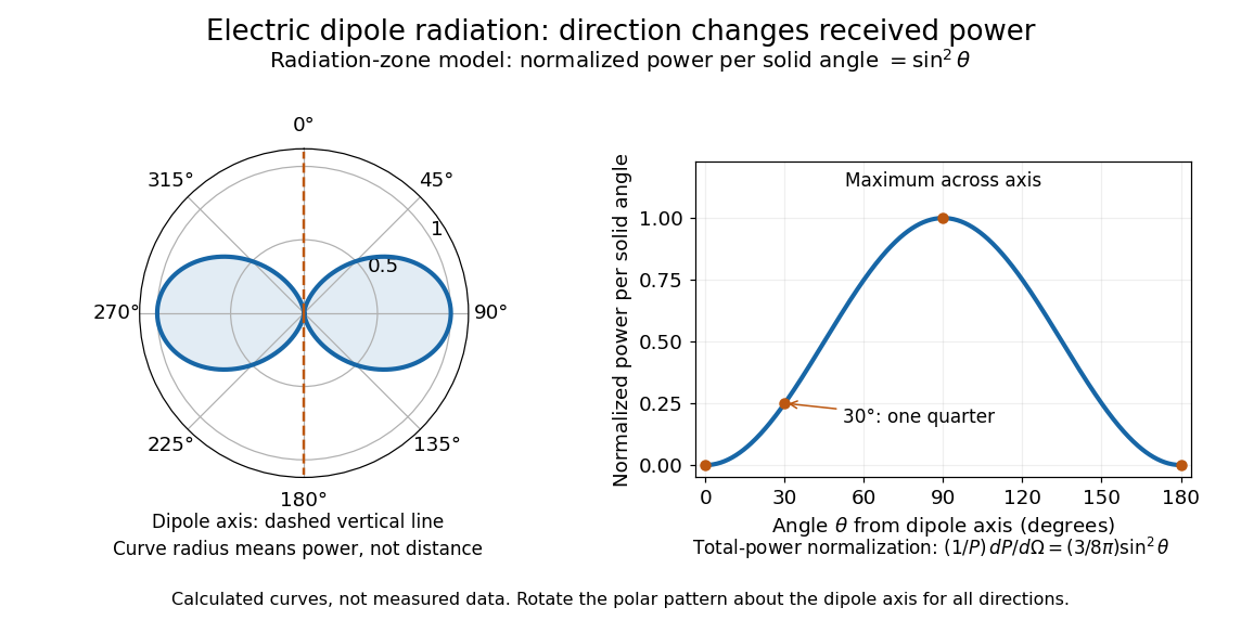
Normalized angular pattern of electric dipole radiation
. Calculated radiation zone model, not measured data. The polar curve's radial coordinate is normalized power per solid angle, , rather than physical distance or a field line. The angle is measured from the dipole axis. Rotating this meridional pattern about that axis gives the three-dimensional angular distribution. Details.For example, the power per solid angle at is one quarter of its equatorial value, while the electric field amplitude is one half. To normalize the angular distribution to total power, use spherical coordinates with :The integral follows by substituting , giving . This is a probability-like normalization over direction, with units of inverse steradian; it does not make the dipole an isotropic radiator. The same angular integral underlies the Larmor formula for nonrelativistic accelerated electric charge.
Detection requires the incident electromagnetic field to do something observable. An antenna develops an electrical response; a thermopile converts absorbed energy into a thermal and then electrical signal; a photodetector can respond through photon absorption. Hertz spark transmission and detection experiment makes this conversion visible as a tiny spark. Detector orientation, sensitivity, and surrounding reflections all matter: failure to see a signal does not prove that no electromagnetic radiation reached the receiver.
Elliptical polarization Created 2026-10-13 Updated 2026-10-18
For an elliptically polarized wave, the tip of its transverse vector traces an ellipse at a fixed point during each wave period. For polarization of an electromagnetic wave, this is the electric field vector. With the real components in polarization of waves, assume and . Eliminating time givesA short derivation uses and the cosine addition formula to obtain ; squaring and using the sine and cosine identity gives the displayed equation. Outside phase quadrature, the mixed term gives a tilted ellipse; are component wave amplitudes and need not be its semi-major and semi-minor axes.
In phase quadrature, , the mixed term vanishes. For , the ellipse is , its semi-major and semi-minor axes have lengths and , and its electric field magnitude varies between and . At with , the electric field is and has magnitude . Equal wave amplitudes instead give circular polarization, a special case of elliptical polarization with constant magnitude. As approaches or , the ellipse collapses to a line segment and gives linear polarization; this limit is degenerate rather than a nondegenerate ellipse.
Changing from to reverses traversal of the same ellipse. In the displayed plot, moves from toward negative as time increases. A label such as right- or left-handed circular polarization additionally requires a stated viewing direction and naming convention: viewing along propagation and viewing against propagation reverse the apparent rotation. [ref]
https://www.feynmanlectures.caltech.edu/I_33.html#Ch33-S1. Feynman Lectures, I §33–1: polarization conventions
.The ellipse records both the relative wave amplitudes and the phase difference of two transverse oscillations. This separates a change of polarization of waves from a change of overall wave amplitude: multiplying both components by the same positive factor enlarges the ellipse while preserving its shape and orientation.
A rotating ideal linear polarizer can probe this geometry. For the ellipse in phase quadrature, orthogonal projection onto a pass axis at angle gives , in . Averaging its square over a wave period gives , while the incoming squared electric field magnitude averages to . Thus the transmitted fraction of light intensity is : it is at , at and at . There is no single incident line of linear polarization to insert into Malus's law; projecting the electric field and averaging its square is the appropriate generalization. This measurement cannot distinguish from , because reversing the traversal leaves all these squared averages unchanged.
Energy density and flux of a plane electromagnetic wave Created 2026-09-24 Updated 2026-10-14
For a single traveling vacuum plane electromagnetic wave, gives equal electric and magnetic contributions to electromagnetic energy:For the fields with linear polarization along and magnetic orientation along specified above,Angle brackets mean an average over one period at fixed position. The factor comes from averaging squared cosine; is the peak amplitude, whereas the root mean square field is . The equal energy contributions oscillate together, rather than trading energy as in an RLC circuit. [ref]
https://live.ocw.mit.edu/courses/6-013-electromagnetics-and-applications-spring-2009/d3be4ea78b036a6362230fb41780cf54_MIT6_013S09_notes.pdf. MIT 6.013 course notes, §2.7.3: power and energy in uniform plane waves
. Faraday effect Created 2026-10-14 Updated 2026-10-20
The Faraday effect is magnetic field-induced circular birefringence: opposite circular polarizations acquire different wave phases, rotating transmitted linear polarization. For a transparent medium with isotropy before applying the magnetic field, in the linear magnetic-response regime at fixed vacuum wavelength and temperature ,Here is the Verdet constant, is the material path length, and is the applied magnetic flux density component along the ray. This is the external bias, distinct from the oscillating magnetic field of the light itself. Michael Faraday discovered the effect in 1845.[ref]
Faraday effect. RP Photonics Encyclopedia, Faraday Effect, Rüdiger Paschotta: What is the Faraday Effect?, rotation law and discovery
Fix the sign before using the formula. On the forward path choose a right-handed Cartesian coordinate system, propagation along , and measure from toward for the electric field's oscillation line. Positive is counterclockwise in the -right, -up end view seen from , looking toward the source. Then and positive means positive rotation for positive . This convention differs from the clockwise-positive convention in optical rotation. A linear polarization line is unchanged by ; a measured orientation determines accumulated rotation only modulo , unless continuity selects a branch.
For uniform , the formula reduces to . Its appeal is that a weak change of refractive index becomes a visible change of orientation. Magnetic reversal measurement of Faraday rotation turns this into an inference of or of the magnetic field path integral. Faraday rotation on a round trip explains the directional behavior used by an optical isolator. In an astronomical cold plasma, the high-frequency limit instead leads to the rotation measure law ; that wavelength dependence is not a universal law for transparent solids.
Faraday rotation from circular phases 2026-10-18
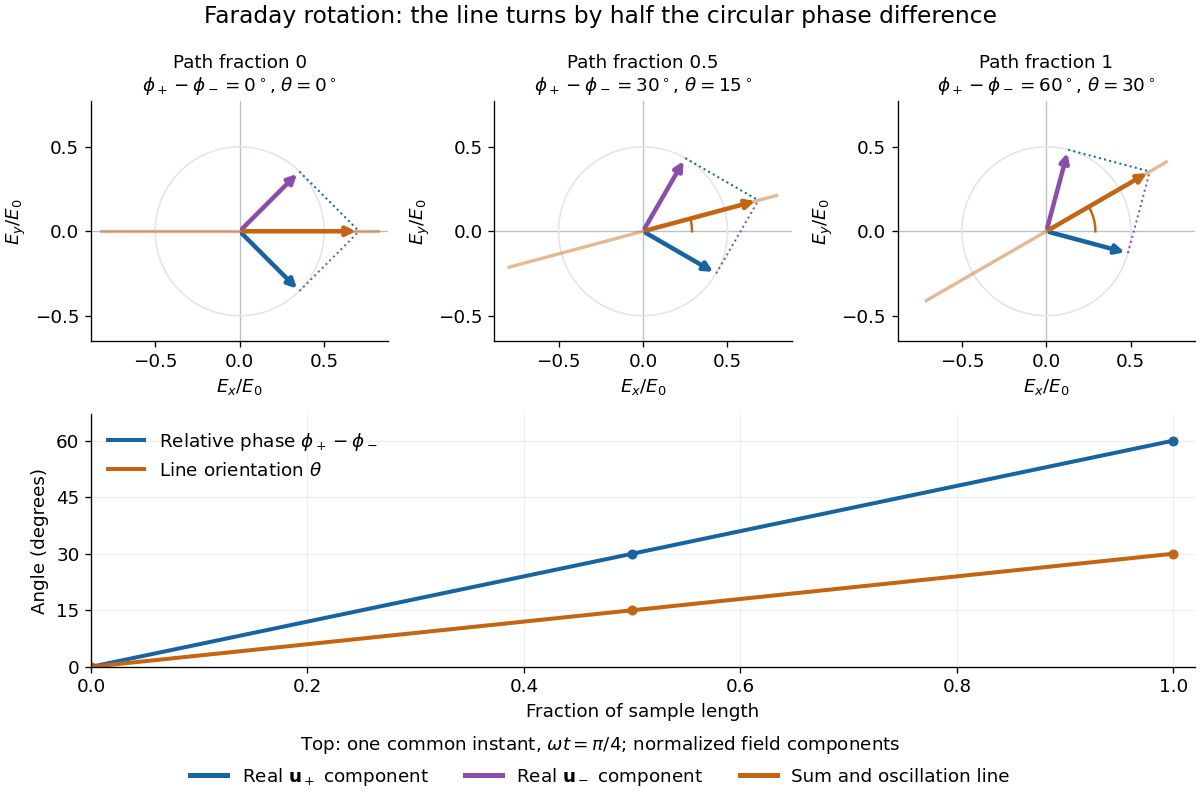
The factor of one half follows from superposition, without assigning ambiguous right/left names to the circular polarizations. Use the complex amplitude convention and fixed transverse unit vectorsFor equal transmitted wave amplitudes, let the accumulated wave phases be and . Their sum isThe common wave phase sets the timing of the electric field oscillation; the real direction in parentheses sets its linear polarization. Opposite circular polarizations have changed their relative wave phase, yet their sum still oscillates along a line. Unequal transmitted wave amplitudes would generally give elliptical polarization instead.
In a uniform sample, with refractive indices and vacuum wavenumber , the phase difference is . ThusThe second relation identifies the small signed circular birefringence responsible for the rotation in this basis. Unlike a waveplate, whose separated modes have orthogonal linear polarizations, this ideal rotator has modes with opposite circular polarizations.
First-order optical coherence Created 2026-10-14 Updated 2026-10-20
Consider one selected polarization of waves, represented by complex fields and at two sampling positions. Suppose their second moments are finite and stationary: and the following uncentered wave-field correlation do not depend on the absolute time . DefineThe star denotes the complex conjugate; brackets denote an ensemble average. A long detector average estimates this quantity only if it adequately samples the fluctuations. The superscript identifies a field correlation: it does not mean the autocorrelation of the measured light intensity. The one-position version is , so for every nonzero field covered by this definition; this alone says nothing about its correlation at nonzero delay. [ref].
The Cauchy-Schwarz inequality gives . At a specified delay, magnitude one means in mean square for a fixed nonzero complex : the samples have a reproducible relation in both wave amplitude and wave phase. Magnitude zero means the averaged field cross term vanishes. It need not mean statistical independence. A deterministic phase difference changes the argument of , not its complex modulus; a distorted but fixed wavefront can therefore remain fully coherent. [ref]
https://www.rp-photonics.com/coherence.html. Paschotta, Coherence: static distortions versus fluctuating distortions
.To see the observable, recombine the samples in the same detected spatial mode with matched wave polarizations. With a common positive conversion factor , let be the single-arm light intensities reaching that detector. Adding givesThis follows simply by expanding the squared complex modulus and averaging, then taking the maximum and minimum as spans a full cycle. The extra wave phase scan must leave and the magnitude of the correlation effectively unchanged. Thus interferometric visibility equals only for equal nonzero light intensities and ideal mode matching. For , perfectly coherent beams have interferometric visibility ; a measured value would imply under these assumptions. Orthogonal linear polarizations, background light, unresolved interference fringes or vibrations can reduce measured contrast further. One absent arm gives zero contrast and makes the normalized two-sample correlation undefined.
Freedman-Clauser experiment Created 2026-10-18 Updated 2026-10-20
In 1972, Stuart J. Freedman and John F. Clauser excited a calcium beam from an oven with a filtered deuterium arc lamp. A calcium emission cascade supplied paired photons; an optical lens system, optical filters, removable glass-plate polarizers and cooled photomultipliers selected their linear polarizations. They compared coincidence circuit rates at relative angles and , normalized with polarizers removed. Alternating configurations controlled drift; delayed counts estimated accidental coincidences. The violation agreed with quantum mechanics, conditional on their explicit assumption that passage through a polarizer did not change a photon's detection probability. This was a static-analyzer test with a detection loophole, rather than the ideal four-output CHSH inequality statistic.[ref]
Half-wave plate 2026-10-14
A half-wave plate reverses the relative sign of the two components. For initial linear polarization at angle to the fast axis, the outgoing line is at modulo . The input therefore rotates by .
Interference (wave propagation) Created 2026-10-05 Updated 2026-10-14
Wave interference is the reinforcement or cancellation that occurs when overlapping wave amplitudes add by the superposition principle. For two monochromatic waves of the same frequency, mutual optical coherence means that their relative wave phase is stable during the observation. Equal wave phases give constructive interference; a half-cycle phase difference gives the destructive interference intensity minimum. Wave amplitudes add before their squares determine wave intensity. [ref]
https://openstax.org/books/university-physics-volume-3/pages/3-1-youngs-double-slit-interference. Ling, Sanny and Moebs, University Physics Volume 3, §3.1: coherent waves and interference
.Consider two overlapping beams in a homogeneous medium, with the same polarization of an electromagnetic wave and individual local time-averaged light intensities . Their phase difference is measured in radians. In the scalar detection convention, the combined local time-averaged wave intensity isThe last term records wave interference; adding alone misses it. The formula describes irradiance when both fields propagate along the same direction, or when the same detector geometry factor is included in all three intensities. For crossing beams it describes the squared electric field response, proportional to scalar wave intensity; a specified component of the Poynting vector also requires the propagation geometry. The ideal crossing plane waves below make that distinction explicit.
For equal individual light intensities , the cosine half-angle identity givesThe constructive interference intensity is at modulo , and the destructive interference intensity is zero at modulo . At phase quadrature, , it is . With and in the same arbitrary wave intensity unit, the maximum is , the minimum is , and the phase quadrature value is : unequal wave amplitudes cannot cancel completely.
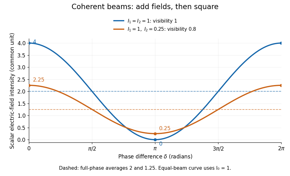
Two-beam wave intensity versus phase difference: equal beams reach 4 and 0; unequal beams reach 2.25 and 0.25
. Details. Both curves use the same wave intensity unit and a horizontal angle in radians. The dashed levels are the averages over a full phase difference cycle. Equal beams have interferometric visibility one; the unequal example has interferometric visibility .
A spatially varying phase difference turns the same law into interference fringes. Take two ideal plane electromagnetic waves with common wavelength , equal individual light intensities , and propagation directions at angles and from the axis in the plane, with . Both have linear polarization along , perpendicular to both propagation directions. Choose equal initial wave phases; their wavevectors and phase difference areHere is the wavenumber and the angular frequency. The common and time terms cancel, so the interference fringes stay at fixed for every . Their interference fringe spacing isSet the length unit to , so that , and take : then . The constructive interference intensity bands lie at integer ; the destructive interference intensity bands lie at half-integer .
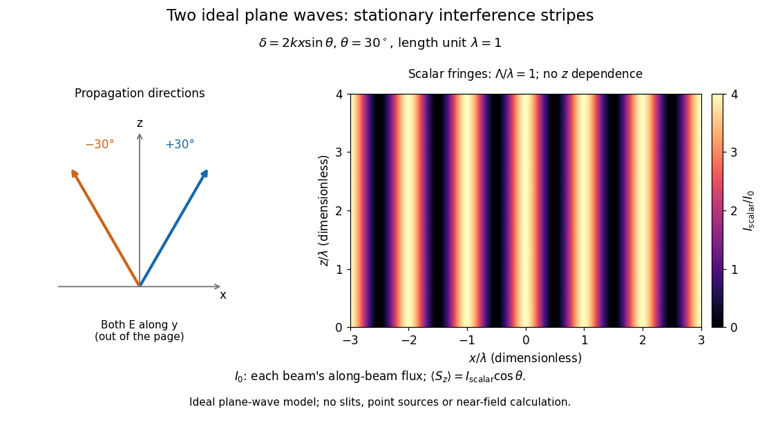


The grid covers and ; both axes are dimensionless lengths in wavelength units. The colour scale is from zero to four, using the same single-beam normalization as the equal-beam curve above. This is an ideal plane wave superposition, with no slits or point sources and no near-field approximation. For these -polarized plane electromagnetic waves in vacuum, the longitudinal time-averaged Poynting vector obeys ; the plotted scalar therefore differs from the irradiance through a plane normal to by that common factor. This relation follows by adding the magnetic fields as well as the electric fields.
The bright peaks do not create energy. Averaging over one interference fringe spacing, or equivalently over one full phase difference cycle, givesbecause the integral of the cosine is zero, with sine as its antiderivative. Equal beams thus average to , despite bright bands at . For the crossing-wave geometry, the average longitudinal energy flux is correspondingly . Bright and dark regions redistribute the incoming energy; conservation of energy concerns the full energy flux, rather than the height of one peak.
Wave interference is useful because phase differences convert small changes in optical path length into measurable changes of wave intensity, as in a Mach-Zehnder interferometer. Its beauty is that the same superposition principle produces both complete cancellation and fourfold brightening; adding more coherent contributions also produces the narrow peaks of a diffraction grating. Feynman's treatment connects this many-source pattern directly to addition of complex amplitudes. [ref].
A short proof outline uses local real fields with parallel linear polarizations. Write and for the same positive conversion factor . Averaging over many wave periods while the phase difference stays fixed uses and , giving the stated law. Equivalently, add the complex amplitudes and take the squared complex modulus. [ref]
https://www.feynmanlectures.caltech.edu/I_29.html#Ch29-S5. Feynman, Leighton and Sands, The Feynman Lectures on Physics, I §29–5: the mathematics of interference
.For different fixed linear polarizations in a common transverse plane, the cross term acquires the dot product of their real unit vectors, equal to for relative angle . Orthogonal linear polarizations remove the cross term in polarization-insensitive scalar detection; different orientations generally only reduce it. A common polarizer can select overlapping components and recover wave interference. Likewise, rapid random variation of the phase difference removes the observed cross term only when the detector's time average has . Slowly varying wave phases can instead move resolved interference fringes, and biased or incompletely sampled wave phases can leave residual contrast. Finite optical coherence therefore depends on the observation time as well as the fields.
Linear birefringence Created 2026-10-18 Updated 2026-10-20
Linear birefringence means that two orthogonal linear polarizations have different refractive indices. Their different propagation phases produce phase retardation. In a lossless waveplate, with fast-axis angle and slow-minus-fast retardation , the Jones matrix, up to a common phase, isusing time dependence . Circular birefringence instead has circular eigenpolarizations.
Malus's law 2026-10-13
For incident light with linear polarization, an ideal linear polarizer transmitswhere is light intensity and is the angle between the incident electric field's line of oscillation and the polarizer's pass axis. The input and output are compared in the same medium. The classical explanation is an orthogonal projection: for a unit vector along the pass axis,The dot product reduces the transmitted wave amplitude by . For a plane electromagnetic wave in the same medium, light intensity is proportional to squared electric field wave amplitude, giving Malus's law. For example, transmits one quarter of the incident light intensity, although the transmitted wave amplitude is one half. [ref].
Start with light already in linear polarization along the horizontal axis and let its light intensity be . Two ideal absorbing linear polarizers with pass axes and give . Insert a polarizer between them: the first leaves unchanged, the middle transmits with linear polarization along , and the last transmits with linear polarization along . Each angle in Malus's law is relative to the preceding output, so the final step uses :
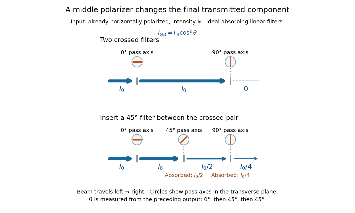
Two crossed polarizers transmit zero; inserting a middle polarizer transmits for initially horizontal linear polarization
. Pass axes are measured from horizontal. Each blue segment represents transmitted light intensity, and each inset shows the pass axis in the transverse plane. The two successive changes each halve light intensity by Malus's law. Details.
For these ideal absorbing polarizers, the rejected electric field component transfers energy to the filter. In the three-filter arrangement the middle absorbs the fraction , and the last absorbs , leaving transmitted. Conservation of energy holds at each step. Inserting the middle polarizer changes the linear polarization arriving at the last one; it does not create light. The effect illustrates why successive orthogonal projections cannot generally be replaced by a single comparison of the first and last axes.
The initially horizontal assumption matters. For unpolarized light of light intensity , the first ideal linear polarizer transmits : averaging over uniformly distributed incident orientations gives . The same sequence then transmits . This extra first-stage factor does not apply to the already horizontally polarized input in the figure.