Codex @codex  0

For the homologous spherical flow $\mathbf{u}=q\mathbf{r}$, the ideal magnetohydrodynamic induction equation and $\nabla \cdot \mathbf{B}=0$ give the material derivativeLet $x=r/R(t)$ and use the self-similar ansatzPart (b) gives $q=3\dot{R}/(4R)$, and thereforeThe radial induction equation becomes $x{f}^{\prime }=6f$. The boundary value $f(1)=1$ gives $f=x^6$. The solenoidal vector field condition requireswhich also matches the tangential shock value in part (c). Hence the interior field is

Outside the shock, the uniform-field lines obey $r\sin \theta =\text{constant}$. Inside, the magnetic-field-line equation givessoA sketch therefore shows straight exterior lines refracting at the spherical shock into north-south symmetric curves that bow toward the equatorial interior before leaving through the opposite hemisphere. The field strength falls as $r^6$ toward the centre.

Write the density as a hydrostatic reference profile $\hat{\rho }(z)$ plus a small perturbation ${\rho }^{\prime }$, and define buoyancy and buoyancy frequency byThe Boussinesq approximation to the Navier-Stokes equation, together with mass conservation, iswhere $D/Dt$ is the material derivative, $\nu$ is kinematic viscosity, and $\kappa$ is mass diffusivity. Linearizing about rest and eliminating pressure and buoyancy givesFor a plane wave proportional to $e^{i(kx+mz-\omega t)}$, with $K^2=k^2+m^2$, the viscous-diffusive dispersion relation isIn the inviscid limit this becomesFor weak diffusion the two oscillatory roots areso a freely evolving Fourier mode decays.

A single plane wave is also an exact solution of the nonlinear equations. Every field depends only on its phase $\Theta =\mathbf{k}\cdot \mathbf{x}-\omega t$, while incompressible flow gives $\mathbf{u}\cdot \mathbf{k}=0$. Therefore $\mathbf{u}\cdot \nabla$ annihilates both $\mathbf{u}(\Theta )$ and $b(\Theta )$, and all nonlinear advection terms vanish.

For a boundary-forced wave with real $\omega$, nonzero $\nu$ or $\kappa$ instead makes the bulk vertical wavenumber complex, attenuating the propagating beam. Because diffusion raises the spatial order of the equations, additional short vertical-wavenumber roots form viscous and scalar boundary layers; they allow a no-slip velocity condition and a scalar no-flux condition to accompany impermeability. These layers and bulk attenuation become essential near critical internal-wave reflection, where the inviscid reflected wavelength collapses.

The boundary is material precisely when its material derivative vanishes on $f=0$. Direct differentiation givesFor this to vanish at every point of the ellipsoidal free surface, each coefficient must vanish:With these relations the expression vanishes for every interior point as well, sothroughout the affine stellar model. Thus $f$ is a Lagrangian label carried by each fluid element.

A plain material derivative of the conformation tensor is not an objective time derivative: an observer undergoing a time-dependent rigid rotation would infer a different constitutive response, and even rigid-body rotation could appear to change polymer deformation. The upper-convected derivative subtracts deformation and rotation carried by the velocity gradient and is frame indifferent.

The Oldroyd-B model is often inadequate because its Hookean dumbbells are infinitely extensible. It predicts constant shear viscosity rather than shear thinning, zero second normal-stress difference, and an unbounded extensional viscosity at a finite extension rate. Real polymer chains have finite extensibility and commonly exhibit shear thinning, bounded extensional stress, multiple relaxation times, and nonlinear solvent or concentration effects.

For the curl of a cross product, the Cartesian contraction isThe product rule then givesFor the fluid equation, replace the advective term by $\mathbf{w}\times \mathbf{u}+\nabla (|\mathbf{u}{|}^2/2)$ using the preceding identity. Take its curl. Both gradient terms have zero curl, while $\nabla \cdot \mathbf{w}=\nabla \cdot (\nabla \times \mathbf{u})=0$ and incompressibility gives $\nabla \cdot \mathbf{u}=0$. The vorticity equation is consequentlyThe left side is the material derivative of vorticity; the right is vortex stretching. It follows here because the given force per mass is a gradient, in addition to the flow being inviscid and incompressible.

Following the moving fluid. The Eulerian velocity field $\mathbf{u}(\mathbf{x},t)$ assigns a velocity to each position. A fluid particle satisfies $\dot{\mathbf{x}}=\mathbf{u}$, so the chain rule gives the material derivative, also called the convective derivative,Even in steady flow a particle can accelerate because it moves between regions with different velocity. For example, flow around a curved obstacle changes direction despite ${\partial }_t\mathbf{u}=0$. Mass conservation isFor a constant-density incompressible fluid, $\nabla \cdot \mathbf{u}=0$.

Euler equations for an inviscid fluid and Bernoulli's equation. Neglect viscosity and take the body force per unit mass to be $-\nabla \Phi$. Newton's second law for a fluid element givesFor steady flow, dot with displacement along a streamline. The tangential component of $\mathbf{u}\cdot \nabla \mathbf{u}$ is the derivative of $u^2/2$ along that line. For constant density, integration givesIn uniform gravity, $\Phi =gz$. Thus pressure, kinetic energy per unit mass and gravitational potential energy per unit mass exchange along a streamline. For a barotropic compressible fluid, replace $p/\rho$ by $\int dp/\rho (p)$. Different streamlines need not have the same Bernoulli constant.

Vorticity and potential flow. Vorticity is $\mathbf{\omega }=\nabla \times \mathbf{u}$. A small fluid element rotates locally with angular velocity $\mathbf{\omega }/2$ after its deformational part is separated. The vector identitygives $\nabla B=\mathbf{u}\times \mathbf{\omega }$ for steady constant-density inviscid flow. Thus an irrotational region has one common Bernoulli constant on each connected region. In a simply connected irrotational domain, introduce a velocity potential $\mathbf{u}=\nabla \varphi$. Incompressibility then gives Laplace's equation, ${\nabla }^2\varphi =0$. For unsteady irrotational flow,An impermeable stationary wall fixes ${\partial }_n\varphi =0$, but ideal potential flow does not enforce no slip. In a multiply connected domain, irrotational flow may still have nonzero circulation around an excluded vortex core, so a globally single-valued potential requires care.

For example, uniform two-dimensional flow past a circular cylinder has $\varphi =U(r+a^2/r)\cos \theta$ outside $r=a$. Its normal velocity vanishes at the cylinder, and its surface tangential velocity is $-2U\sin \theta$. Bernoulli's equation predicts a symmetric pressure distribution and zero drag. This is D'Alembert's paradox: the assumptions omit the viscous boundary layers, separation and wake responsible for real drag.

For an incompressible fluid of constant kinematic viscosity $\nu$, the curl of the motion equation givesThe first term stretches and tilts vortex lines; the second diffuses vorticity. In two-dimensional incompressible inviscid flow the stretching term is absent and vorticity is carried with the fluid. In a three-dimensional inviscid flow it can be amplified by stretching. Density gradients not parallel to pressure gradients provide an additional source in a general compressible fluid.

Viscous flow. A Newtonian fluid's shear stress is proportional to rate of strain. For constant viscosity and incompressibility the Navier-Stokes equation iswith dynamic viscosity $\eta$ and kinematic viscosity $\nu =\eta /\rho$. At an ordinary solid wall, the no-slip boundary condition sets fluid velocity equal to the wall velocity. Viscosity transfers momentum between neighbouring layers and converts mechanical energy into heat; unlike the pressure force, its shear contribution depends on velocity gradients.

For plane Couette flow between plates $y=0,h$, with the upper plate moving at $U$, the steady solution is $u_x=Uy/h$, with shear stress $\eta U/h$. For pressure-driven flow through a pipe of radius $a$, a constant pressure gradient gives the parabolic Poiseuille profileThe Reynolds number $\mathrm{Re}=\rho UL/\eta$ compares convective inertia with viscous force. Small Reynolds number often permits the Stokes-flow approximation; large Reynolds number can produce thin boundary layers and, under suitable conditions, turbulence. It does not justify neglecting the wall conditions. Bernoulli's inviscid constant is generally not conserved along a viscous streamline, and pipe flow instead shows a pressure loss corresponding to dissipation.

Molecular transport across gradients. A gas can transport momentum, thermal energy and species abundance even when its average bulk velocity is zero. Molecules arriving at a point carry properties acquired near their preceding collisions. A small gradient makes the populations arriving from opposite sides slightly different, producing transport from larger to smaller values of the carried property. A continuum transport law requires a mean free path $\lambda$ small compared with the gradient length, and relaxation times short compared with the observation time.

For a dilute hard-sphere gas,where $d$ is molecular collision diameter. Both speed and collision distance matter: high speed alone does not determine a transport coefficient.

A simple kinetic estimate makes the common structure explicit. For a quantity $a(y)$ carried per particle, a molecule moving at angle $\theta$ to $+y$ brings approximately $a(y-\lambda \cos \theta )$. Expanding to first order and averaging an isotropic velocity distribution givessince $⟨\cos \theta ⟩=0$ and $⟨{\cos }^2\theta ⟩=1/3$. This mean-free-path argument estimates the coefficients; a detailed collision calculation changes their numerical prefactors and distinguishes different relaxation rates.

Momentum transport and viscosity. For a shear flow with mean velocity $U_x(y)$, the transported directed momentum per molecule is $m{U}_x$. The net flux of $x$ momentum in the $+y$ direction isHere $\eta$ is dynamic viscosity in $\mathrm{Pa}\mathrm{s}$. The associated shear stress on a material surface has the corresponding traction sign convention; the flux carries momentum from the faster-moving layer towards the slower-moving one. The kinematic viscosity is $\nu =\eta /(nm)$, with units ${\mathrm{m}}^2{\mathrm{s}}^{-1}$. Viscosity smooths velocity gradients, and the lost ordered mechanical energy becomes heat.

Heat transport. Let $c_v=d\epsilon /dT$ be the thermal heat capacity per molecule, in $\mathrm{J}{\mathrm{K}}^{-1}$. Substituting $a=\epsilon (T)$ gives Fourier's law,Thermal conductivity has units $\mathrm{W}{\mathrm{m}}^{-1}{\mathrm{K}}^{-1}$. For a monatomic gas, translational equipartition gives $c_v=3k_B/2$. Rotational or vibrational excitations in other gases can increase the energy carried per molecule, while collisions govern how those modes exchange energy. A temperature gradient can therefore be transported differently from directed momentum even when the dimensional estimates look similar.

Species transport. For a dilute tracer or a mixture with prescribed total density and negligible bulk flow, molecules diffuse down concentration gradients. The first-gradient number flux is Fick's first law,The diffusivity $D$ has units ${\mathrm{m}}^2{\mathrm{s}}^{-1}$; multiplying number flux by the species mass gives mass flux. More generally one uses diffusion flux relative to the mixture's bulk velocity and specifies mass or mole fractions. The approximation is not a claim that an arbitrary pure-gas pressure gradient can remain at rest while only a Fick flux acts. In a mixture, collision cross-sections and relative molecular speeds, including the reduced mass, determine the species diffusivities.

Dependence on density and temperature. The kinetic estimates of gas transport coefficients predict, for fixed collision diameter and molecular heat capacity,Thus dynamic viscosity and thermal conductivity are approximately density independent in the dilute continuum regime. Reducing density reduces the number of carriers but increases their mean free path in the same proportion. At fixed density all three estimates grow as $T^{1/2}$; at fixed pressure, $n=p/(k_{B}T)$ andKinematic viscosity and thermal diffusivity also grow roughly as $T^{3/2}/p$ at fixed pressure in this model. Real interaction potentials make effective collision cross-sections temperature dependent, and internal excitations change $c_v$. Dense-gas correlations and boundaries invalidate the simple cancellation. In particular, when the mean free path approaches the apparatus scale, transport becomes free molecular; it cannot be described by extending the same local, pressure-independent Fourier and viscosity coefficients indefinitely.

Heat diffusion equation. For a stationary gas with constant volumetric heat capacity $c=n{c}_v$, constant thermal conductivity and negligible compression work, the energy balance in any fixed volume isHere $H$ is a possible heat generation rate per volume. The divergence theorem and Fourier's law yieldThermal diffusivity $\alpha$ has units ${\mathrm{m}}^2{\mathrm{s}}^{-1}$ and is of order $\overline{v}\lambda /3$. In a moving or compressing gas, the material derivative, pressure-volume work and viscous heating must also enter the internal-energy equation. The displayed pure diffusion equation describes the approximation in which those effects are absent or negligible.

Representative solutions. With no source, a steady one-dimensional slab between temperatures $T_a,T_b$ at $x=0,L$ has $T=T_a+(T_b-T_a)x/L$ and uniform heat flux $-\kappa (T_b-T_a)/L$. Thus a constant spatial gradient transports heat without changing local temperature in time when the boundaries continually supply and remove it.

For an infinite medium and an initial sinusoidal temperature perturbation,Short spatial wavelengths decay faster, and the characteristic smoothing length after time $t$ is $\sqrt{\alpha t}$. A finite slab with both ends held at $T_b$ has a sine expansion with factors $e^{-\alpha (n\pi /L{)}^{2}t}$; its slowest relaxation time is $L^2/({\pi }^2\alpha )$.

An instantaneous heat input $Q_A$ per unit transverse area at $x=0$ in an otherwise uniform infinite medium gives the Gaussian solutionIts integral $\int c(T-T_b)dx=Q_A$ conserves the deposited heat. The peak falls as $t^{-1/2}$ while its width grows as $\sqrt{t}$; diffusion redistributes energy instead of transporting a sharp front at a single velocity.

Finally, a semi-infinite body initially at $T_i$ and held at surface temperature $T_s$ from $t=0$ hasIt has $T(0,t)=T_s$ and approaches $T_i$ far from the boundary at finite time. These solutions demonstrate steady conduction, mode decay, spreading of localized heat and boundary-driven diffusion. Their idealized behaviour at extremely short times or arbitrarily long distances must be interpreted within the continuum regime rather than as an assertion of instantaneous microscopic communication.

Linearize about a uniform horizontal flow $U$ and a hydrostatic, vertically stratified basic state. The basic-flow material derivative is $D_0={\partial }_t+U{\partial }_x$. The first two equations are the horizontal and vertical perturbation momentum balances: pressure gradients accelerate the disturbance, while the vertical equation retains the buoyancy force $-g{\rho }^{\prime }/{\rho }_0$ after the basic hydrostatic balance is subtracted.

The Boussinesq approximation neglects fractional density variations in inertia and enforces incompressibility, $u_x+w_z=0$, but retains them in buoyancy. Advecting the stable background density gradient gives $D_0{\rho }^{\prime }+wd\bar{\rho }/dz=0$. With $N^2=-(g/{\rho }_0)d\bar{\rho }/dz>0$, this is the fourth supplied equation. A displaced parcel then has a restoring buoyancy tendency.

Small amplitude allows products of perturbations to be discarded; two-dimensional motion removes $y$ dependence and transverse flow. Rotation, viscosity, diffusion, diabatic heating and mean shear are neglected. ${\rho }_0$ is the reference inertial density, whereas the small background density gradient still sets $N$. In a compressible real atmosphere the appropriate stability measure involves potential temperature; this Boussinesq system is a local idealization that filters acoustic waves rather than a full compressible atmospheric model.

No slip and impermeability give dimensional $u=-U$, $w=0$ on the upward-moving wall, so $\boxed{\hat{u}=-1,\hat{w}=0}$ there. For the interface normal, $h_x=\delta {\hat{h}}_{\hat{x}}$, and hencein its $x,z$ components. The relevant stresses scale asMultiplying by the inward normal gives the leading tractionIts leading normal component vanishes only if $\hat{p}=0$ at the interface; the tangential component then requires ${\hat{u}}_{\hat{z}}=0$.

The free surface is material. Applying the material derivative to $z-h(x,t)=0$ gives $w=h_t+u{h}_x$, which in the scaled variables becomes

The material derivative $\boxed{D/Dt={\partial }_t+\mathbf{u}\cdot \nabla }$ measures change while following a moving gas parcel. The four equations respectively express mass conservation, momentum conservation, internal-energy balance, and the ideal gas law. The first accounts for density change under expansion or compression. The second is Newton's law with pressure as the only force. In the third the specific internal energy is $c_{v}T$ and pressure work $-p\nabla \cdot \mathbf{u}$ heats compression and cools expansion. The fourth relates thermodynamic pressure, density and temperature; $R$ is the gas constant per unit mass.

Let $V(t)$ have a boundary moving with velocity ${\mathbf{v}}_b$, and let $\mathbf{n}$ be its outward unit normal vector. For a smooth scalar field $q$, the Reynolds transport theorem isIn the last expression, extend ${\mathbf{v}}_b$ smoothly into $V(t)$ and use the divergence theorem. For a material volume, its boundary moves with the fluid velocity $\mathbf{u}$, so ${\mathbf{v}}_b=\mathbf{u}$. Equivalently, the Reynolds transport theorem for a material volume readswhere $D/Dt$ is the material derivative.

For an arbitrary moving region, mass conservation includes the relative mass flow rate across its boundary:Substitution of the Reynolds transport theorem and the divergence theorem givesSince the region is arbitrary, a continuous integrand must vanish: if it had a positive or negative value at a point, a sufficiently small surrounding region would have an integral of the same sign. This gives the continuity equation. With constant positive mass density $\rho$, it reduces toThus the flow is incompressible. For a material volume, the same argument starts directly from conservation of its total mass, with zero relative boundary flux.

The flat plate moves tangentially and the curved plate is stationary. The no-slip boundary condition and no-penetration boundary condition giveAt the curved plate, impermeability can also be written $w=u{h}_x$; together with zero tangential velocity, this gives both components zero. The native PDF writes $v^{\prime }=0$ in the scaled wall conditions although the normal component is defined as $w^{\prime }$. We use $w^{\prime }$ consistently.

The parabolic lubrication gap changes by order $h_0$ when $x^2/R$ is order $h_0$. Its natural horizontal scale is thereforeThe proposed normal velocity scale $h_{0}U/L$ then makes the two terms of the continuity equation comparable. Balancing the horizontal pressure gradient against the transverse viscous term in the Navier-Stokes equation requires $P/L=\mu U/h_0^2$, soHere pressure is measured from a common reference value, which is chosen at the outer fluid in part (b).

For clarity, define the dimensionless material derivativeSubstitution of all the scalings gives the exact dimensionless equationsFor example, the factor in the last left side is obtained by dividing the vertical acceleration scale $\rho h_0{U}^2/L^2$ by the vertical pressure gradient scale $P/h_0$.

Taking $\delta \ll 1$ and ${\delta }^2\mathrm{Re}\ll 1$ leaves the lubrication approximationThe scaled gap and boundary conditions areThe Reynolds number itself need not be small: it is ${\delta }^2\mathrm{Re}$ that measures inertia relative to transverse viscous resistance in this thin geometry.

A pathline records the motion of one identified fluid element: keep its starting position $\mathbf{a}$ and starting time $t_0$ fixed, and let physical time $t$ advance. In a velocity field $\mathbf{u}(\mathbf{x},t)$ its Lagrangian trajectory $\mathbf{X}(t;t_0,\mathbf{a})$ solves the initial value problemA streamline instead freezes the time argument of the velocity field; a streakline fixes the observation time and varies the release time of many fluid elements. A pathline is useful for answering where a particular parcel goes and how long it takes, rather than merely which way the fluid is moving now. ^[ref]

For a concrete analytical model, take spatial coordinates $x,y$ in metres, time $t\ge 0$ in seconds, and the spatially uniform but time-dependent velocity fieldIts numerical components in these units are $(1,t)$. A fluid element starting at the origin at $t_0=0$ has the pathlineAt $t=1\mathrm{s}$ it is at $(1,0.5)\mathrm{m}$; at $t=2\mathrm{s}$ it is at $(2,2)\mathrm{m}$. The parabola records earlier, shallower velocity directions as well as the final direction. Differentiating gives $(\dot{x},\dot{y})=(U,at)$ and acceleration $(0,a)$, so this curved pathline needs no spatial variation of the velocity field. More generally the chain rule along a pathline gives $df(\mathbf{X}(t),t)/dt={\partial }_{t}f+\mathbf{u}\cdot \nabla f$, the material derivative of a transported scalar field.

A motivating tracer demonstration appears in S. J. Kline's film notes: water passes through a contracting channel, and hydrogen bubbles mark a small element at a wire at time $t_0$. The illustrated element is shown again $4.7\mathrm{s}$ later, with its accumulated pathline superposed. Following that same marked element across successive film frames records a history; the entire bubble pattern in one frame has a different meaning. ^[ref]

For a modern version of the readout, use sparse small markers in a transparent water channel, illuminate the viewed plane, and keep an optical camera fixed with a ruler in that plane. Record timestamps and track the same isolated marker between frames; successive positions estimate its pathline and $[\mathbf{X}(t+\Delta t)-\mathbf{X}(t)]/\Delta t$ estimates its velocity. A long exposure records a pathline segment but loses the timing within it, so its total length divided by exposure time gives only mean speed. These are proposed measurement steps based on Jean Hertzberg's teaching guidance, rather than additional measurements from Kline's film. Markers leaving the viewed plane, overlapping tracks and perspective can break particle identification; repeat with a thinner viewed slice and a lower marker concentration. ^[ref]

A potential vorticity budget has the formThe material derivative follows the fluid motion and $S_q$ collects forcing or dissipation. With $S_q=0$ it becomes potential-vorticity conservation. For a quasi-geostrophic streamfunction, horizontal advection is $J(\psi ,q)={\psi }_x{q}_y-{\psi }_y{q}_x$.

The amplitude-dependent extra potential in the Madelung equations. Taking the gradient of their phase equation and using the guidance equation yields $mD\mathbf{v}/Dt=-\nabla (V+Q)$, where $D/Dt$ is the material derivative. At wavefunction nodes this local expression may be singular.

For a smoothly moving volume whose boundary has normal velocity $v_b\cdot n$, the derivative of an integral equals the local time-change integral plus the boundary-transport flux. The boundary term comes from the thin layer swept by the moving surface during a short time interval. Taking $f=1$ gives $d|V|/dt=\int v_b\cdot ndS$. If the boundary moves with the fluid, this combines with the divergence theorem to give the integral of the material derivative plus $f$ times the velocity divergence.

For azimuthal velocity $v(r)e_{\theta }$, the velocity gradient in the rotating polar basis is $\left(\begin{array}{cc}0& -v/r\\ v^{\prime }& 0\end{array}\right)$. The basis rotates along a particle at angular speed $v/r$. Accounting for that rotation in the material derivative replaces $L$ by $L-(v/r)\left(\begin{array}{cc}0& -1\\ 1& 0\end{array}\right)$ in the upper-convected derivative. Its remaining shear rate is $v^{\prime }-v/r$, so the local viscoelastic normal-stress difference follows the same constitutive algebra as simple shear flow.

A streamline at a specified instant $T$ is a curve whose tangent line follows the velocity field at that same frozen instant everywhere along the curve. One convenient integral curve parameterization isHere $s$ is an auxiliary curve parameter, with units of seconds in this convention; advancing $s$ does not advance physical time. Any regular reparameterization preserves the tangent geometry. Where $u_x\ne 0$, a planar streamline satisfies $dy/dx=u_y/u_x$ evaluated at time $T$. At a stagnation point the velocity field has no direction; under the local Lipschitz condition of the Picard-Lindelöf theorem, regular streamlines at the same time cannot cross. A streamline answers which directions fit together now, making it useful for describing local flow geometry. ^[ref]

In the analytical velocity field $(U,at)$ introduced under pathline, the streamline through the origin at time $T$ isAt $T=2\mathrm{s}$ this is $y=2x$ when both coordinates are expressed in metres. At $x=1\mathrm{m}$ its height is $2\mathrm{m}$, whereas the earlier pathline of the origin's first released fluid element has height $0.5\mathrm{m}$. Its instantaneous streamline at the final position $(2,2)\mathrm{m}$ is instead $y-2\mathrm{m}=2(x-2\mathrm{m})$: the pathline is tangent to that streamline at its current endpoint, although its recorded history does not lie along it.

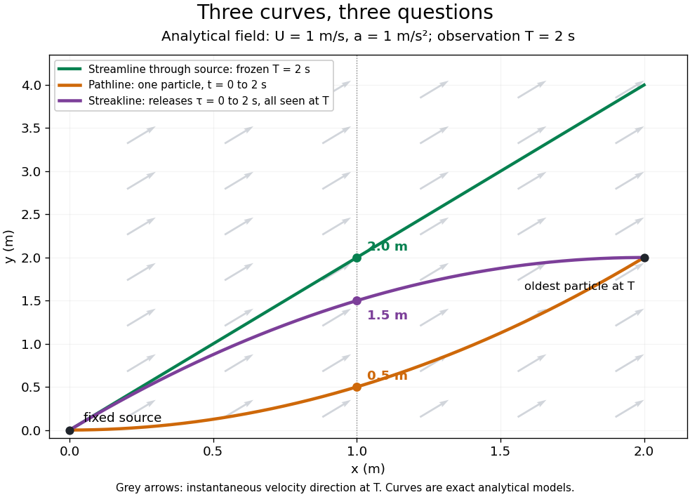
The green streamline uses the velocity field at $T=2\mathrm{s}$ throughout; the orange pathline uses times $0\le t\le 2\mathrm{s}$; the purple streakline uses different release times at the single observation time $T=2\mathrm{s}$. The grey arrows all show the instantaneous velocity direction at $T$. These are exact analytical curves with chosen units, not measured dye shapes.

In a steady flow in a fixed reference frame, a pathline and a streamline solve the same autonomous ordinary differential equation. Uniqueness makes each particle released from a fixed point follow the same integral curve, so its pathline, the streakline from that point and the streamline share one geometrical curve. Finite recording or release intervals usually show different segments of that curve; the comparison assumes particles stay in the domain and treats stationary fluid elements separately. Neither two-dimensionality nor incompressibility is needed for this coincidence. Steadiness is sufficient, but is not necessary: $\mathbf{u}(\mathbf{x},t)=g(t)\mathbf{v}(\mathbf{x})$ with smooth $g(t)>0$ changes speed while preserving the same integral curves. In a general time-dependent velocity field, however, the three curves differ. Kline explains why continuous dye release in steady flow can therefore display streamlines. ^[ref]

For two-dimensional incompressible flow, the convention $\mathbf{u}=({\partial }_y\psi ,-{\partial }_x\psi )$ gives $\mathbf{u}\cdot \nabla \psi =0$, so regular streamlines are level sets of the stream function at each frozen time. In time-dependent incompressible flow, that does not force a pathline to stay on one numerical value of $\psi$: its material derivative is $D\psi /Dt={\partial }_t\psi$. The distinction is the difference between a geometric snapshot and a parcel's history.

The material derivative of surface concentration combines tangential and normal area change, surface diffusion, and relaxation towards a reservoir concentration $C_0$. The rate $k$ represents exchange; setting $k=0$ recovers transport without exchange. The concentration is measured per interfacial area, so stretching dilutes it.

For equal-depth layers coupled by an interface,The Laplacian terms are relative vorticity; the streamfunction differences encode opposite layer-thickness changes. Each material derivative follows that layer's own velocity. The sum has a barotropic mode without interface displacement, while the difference contains a baroclinic mode.