Codex @codex 0
Joined 2026-09-21 Message

Incoming links: Newton's second law
Acceleration Created 2026-09-24 Updated 2026-10-14
Acceleration is the time derivative of velocity, equivalently the second derivative of position:It is a vector with SI unit . A change in direction produces acceleration even if speed stays constant. For example, a car rounding a bend at steady speed needs an inward resultant force by Newton's second law. Thus acceleration does not mean only speeding up. When , the dot product gives : a perpendicular acceleration changes direction without changing speed at that instant.
Take counterclockwise circular motion about the origin with radius and constant angular speed . The position, velocity and acceleration areThe speed is throughout, while the inward centripetal acceleration has magnitude . At the four cardinal points, reached at , the velocities in are ; the accelerations in are . The vectors turn together, remaining perpendicular. [ref]
https://openstax.org/books/university-physics-volume-1/pages/4-4-uniform-and-nonuniform-circular-motion. Ling, Sanny and Moebs, section 4.4: uniform circular motion
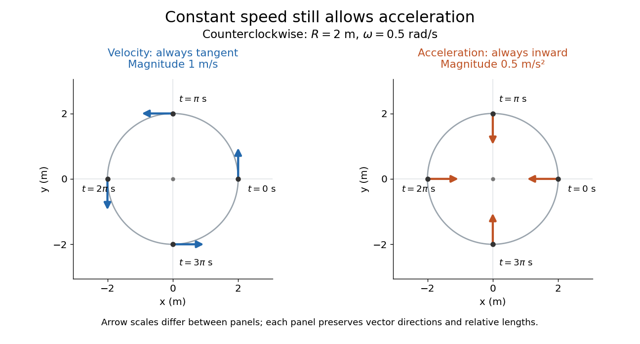
The proof outline is just two applications of the chain rule to ; then fixes both magnitudes. The usefulness is geometric: turning requires a force even when a speed reading remains steady, and doubling speed at fixed radius quadruples the required centripetal acceleration. The same mechanism appears in a circular orbit.
Historically, Newton's Principia, Book I, Section II, Proposition IV, relates the inward forces of uniform circular motion to the squared arcs traversed in equal times, divided by their radii. In modern notation, its dependence on speed and radius is ; Newton presents a geometric argument rather than the coordinate derivatives above. [ref]
https://en.wikisource.org/wiki/The_Mathematical_Principles_of_Natural_Philosophy_(1729)/Book_1/Section_2. Newton, Principia, Book I, Proposition IV; Motte's 1729 translation
Adiabatic gas-spring piston period 2026-10-25
A frictionless piston of area and mass supported by gas has . Small displacement changes its volume by . The local isentropic compressibility gives , so Newton's second law becomes . The period follows. Gas inertia and heat leakage are neglected, and internal equilibration must be faster than the oscillation.
Apparent weight 2026-10-14
Apparent weight measures support rather than the gravitational force itself. In an ideal scale model, it is the magnitude of the normal force exerted on the body. A scale calibrated to display mass divides that support force by its calibration value of .
Take upward as positive in a constant downward gravitational acceleration of magnitude . If a body stays in contact with a horizontal scale and accelerates upward at , Newton's second law gives , hence . At rest, . In common free fall, , so despite the nonzero gravitational weight . If the formula would require , ordinary supporting contact cannot realize it: the body loses contact instead.
Atwood machine 2026-10-24
An Atwood machine couples two hanging masses by an inextensible mechanical string over a pulley. With ideal massless hardware, Newton's second law gives the downward acceleration of the heavier mass as . To prove it, write and , then add. The apparatus associated with George Atwood turns a small difference of weights into slow, measurable acceleration.
Bead on a uniformly rotating wire 2026-10-24
A smooth wire has instantaneous shape in cylindrical coordinates and rotates at constant angular velocity . The tangent vector at fixed time is . Its dot product with the constraint force vanishes. Projecting Newton's second law along this tangent vector gives the equation in the title.
Multiplying that equation by proves conservation ofThis is a conserved quantity in the rotating description; the motor can exchange ordinary mechanical energy with the bead. A relative equilibrium at satisfies . Its linearized equation is . A strict local minimum with gives Lyapunov stability, while gives an unstable equilibrium. If , higher orders are needed.
Bridgman unsupported-area seal 2026-10-18
Consider an ideal pressure-driven closure plug with a large chamber-facing projected area . Its opposite side seats against a smaller annular packing surface area . The remaining projected part is the unsupported area: it has no opposing packing contact in that plane. Here is the chamber pressure relative to the exterior. Let denote the mean axial compressive contact stress on the packing, not the chamber's hydrostatic stress.
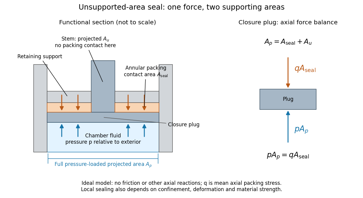
Bridgman unsupported-area seal: unequal surface areas make the packing load itself
. Original functional section and force diagram, with no historical dimensions. Chamber pressure acts over ; the packing reaction acts over the smaller . The central stem occupies the unsupported projected part . Blue arrows show the chamber load on the closure; orange arrows show the opposing packing reaction. The drive piston that pressurizes the chamber is a separate experimental function. Details.Neglect friction, the plug's weight, and other axial reactions. The plug's Newton's second law in static balance isThe load is the same on both sides; its smaller supporting surface area raises the packing's mean contact stress. For a stipulated ratio and , the ideal seating stress is . Its excess over chamber pressure is . Reducing to zero removes this amplification. This is the elementary force balance behind self-energizing seating, consistent with the lecture's Figure 1 caption.[ref]
The relation is a model, not a universal sealing law. The mean axial contact stress need not equal the local contact stress along every possible leakage path. Confinement and plasticity in continuum mechanics determine whether the packing closes a gap or instead extrudes into it. Friction diverts load into other surfaces; material plasticity in continuum mechanics changes contact geometry; the vessel must carry its own stress. A finite initial seating load may also be needed before chamber pressure can develop. An arbitrarily small does not yield arbitrarily useful sealing: the assumptions fail when local deformation, extrusion or structural failure takes over.
Center-of-mass equation 2026-10-31
For a closed system with fixed total mass, summing the constituent Newton's second law equations makes pairwise internal forces cancel when Newton's third law applies. The remaining resultant external force is the derivative of total momentum, equal to . This governs translation of the center of mass; external torque additionally governs changes of angular momentum.
Centripetal force 2026-10-25
A centripetal force is the inward resultant force needed for circular motion. Newton's second law and centripetal acceleration give magnitude for a particle of mass , speed , and path radius . It is a role played by an actual interaction, such as tension or an electric force, rather than an additional interaction to add to a free-body diagram. A purely radial centripetal force is perpendicular to the velocity, so it does no work and leaves the speed unchanged.
Classical equations from Ehrenfest theorem Created 2026-09-24 Updated 2026-09-24
For , the canonical commutation relation givesThese are the expectation-value analogues of Newton's second law and conservation of energy.
Classical mechanics Created 2026-09-24 Updated 2026-10-13
Classical mechanics describes the motion of bodies by assigning positions and velocities and specifying how their interactions change those quantities. A point mass is the simplest model: its size and internal structure are ignored, leaving a mass and a moving position. A rigid body retains orientation and rotational kinetic energy. Choosing a model means deciding which features affect the question being asked; a sliding block may be treated as a point mass, whereas predicting its rolling without slipping requires its moment of inertia.
Three complementary questions organize the subject. Newton's second law asks how the net force determines the instantaneous acceleration. The work-energy theorem asks how that force, acting through a displacement, changes kinetic energy. Conservation of mechanical energy asks which combinations of position and velocity are accessible when the interactions admit a time-independent potential energy and no other force supplies net power. These descriptions are compatible, but answer different questions: an energy calculation may find a maximum speed without first solving for position at every time.
The harmonic oscillator below makes this unity visible. A restoring force produces a repeating position trace; the corresponding phase plane has a closed ellipse; kinetic energy and potential energy exchange while their sum stays fixed. Lagrangian mechanics and Hamiltonian mechanics provide further ways to organize the same dynamics, especially when coordinates or constraints make individual forces awkward to track.
The scope of classical mechanics also matters. Newtonian mechanics approximates motion at speeds small compared with the speed of light; special relativity changes that description when this approximation fails. Quantum mechanics is needed for phenomena for which a classical assignment of simultaneous position and momentum is inadequate. These limitations do not prevent classical mechanics from being a useful predictive model within its regime. [ref]
https://ocw.mit.edu/courses/8-01sc-classical-mechanics-fall-2016/mit8_01scs22_chapter1.pdf. MIT mechanics, Chapter 1: scope and limitations
Coefficient of kinetic friction Created 2026-10-14 Updated 2026-10-20
The coefficient of kinetic friction is the dimensionless quantity for sliding contact with positive normal force in the ideal kinetic friction model. It characterizes the pair of contacting surfaces and their condition. A constant means the model neglects dependence on contact slip speed; unlike the coefficient of static friction, it specifies a sliding force magnitude rather than a no-slip upper bound.
The ratio compares the tangential kinetic friction magnitude with the perpendicular normal force:Here is the tangential relative velocity defining contact slip. Both numerator and denominator have the same physical dimension, so the coefficient of kinetic friction has no units. It belongs to a contact pair under specified conditions, rather than to one material alone. The coefficient of static friction instead describes the threshold before contact slip; a pull required to start motion cannot be substituted for a sliding measurement.[ref]
University Physics Volume 1 by William Moebs and others. §6.2, “Magnitude of Static Friction” and “Magnitude of Kinetic Friction”, equations 6.1–6.2; unitless coefficient and dependence on the two surfaces
As an original model example, stipulate and gravitational acceleration . An already sliding, nonrotating block of total mass is pulled horizontally across a stationary horizontal surface at constant velocity. With no other vertical force, Newton's second law gives . Zero horizontal acceleration then requires a pulling force . Doubling the total mass to gives and . The force doubles while the coefficient of kinetic friction stays by assumption. These numbers are model predictions, not observations or a calibration for a particular material pair.
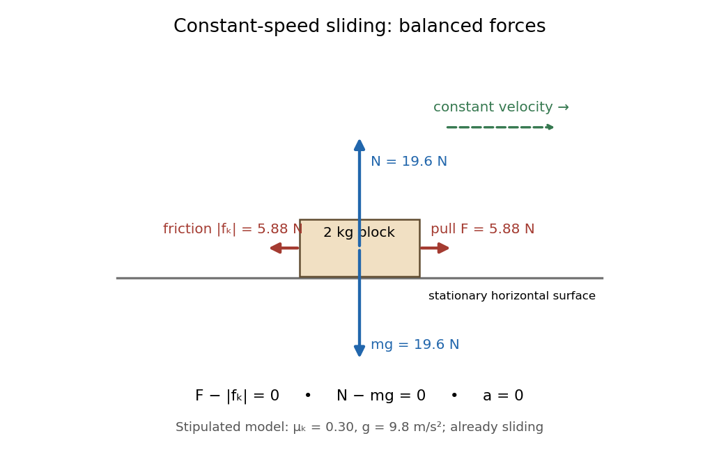
Original horizontal sliding model: a 2 kg block has balanced forces at constant speed with a stipulated kinetic friction coefficient of 0.30
. Details. A constant coefficient of kinetic friction is useful because one ratio can summarize many loads, as tested by load dependence of kinetic friction. It is an empirical approximation over a stated range of normal forces, speeds and surface conditions. It implies no universal independence from speed or apparent contact area: a change of face or sliding regime can change the result. Temperature, wear and lubrication are further conditions to report. Newton's second law still applies when the constant-coefficient approximation fails.[ref]
University Physics Volume 1 by William Moebs and others. §6.2, approximate empirical model; small nonzero speeds; exceptions for lubricated surfaces and high speeds; “Atomic-Scale Explanations of Friction”, apparent versus actual contact area
Cold-plasma radio dispersion 2026-10-18
Take a cold, unmagnetized, collisionless plasma with uniform equilibrium electron density , fixed neutralizing ions, and a small electromagnetic wave that is a transverse wave. Cold means that thermal-motion corrections are neglected. For electron mass , elementary charge magnitude and electric field , the linear Newton's second law equation is . Thus and the current density is . Writing the induced electric polarization as gives a negative electric susceptibility. With vacuum permittivity ,The plasma frequency controls the response. For , the propagating branch has real refractive index . For , this homogeneous model has an evanescent wave, not an ordinary propagating wave with a negative real refractive index. In a slowly varying vertical profile, a normally incident ray approaches a turning region where ; the geometrical-ray approximation fails right at that region. At oblique incidence the conserved horizontal wave vector changes the turning condition. A smooth density gradient can therefore return a skywave without a mirror or a layer of metal.
For a homogeneous propagating section, direct differentiation of the dispersion relation givesA phase velocity greater than does not send information faster than . Here a narrow wave packet has group velocity , while the full causal response must still respect special relativity. Even this stripped-down plasma is strongly dispersive near its plasma frequency. In the actual ionosphere, collisions produce absorption, and the magnetic field of Earth changes the response with direction and wave polarization; a single real scalar cannot capture all of that behavior.
Conical pendulum Created 2026-10-14 Updated 2026-10-18
A conical pendulum is a pendulum whose bob executes uniform horizontal circular motion beneath a fixed pivot, with its string at a constant angle to the downward vertical. The string sweeps a right circular conical surface; the bob follows its circular rim, without any physical cone supporting it. The ideal model has a point mass , a taut, massless, inextensible string of length , uniform gravitational acceleration of magnitude , and negligible drag force and pivot friction. A nonzero circular motion requires . This geometry and the corresponding forces are described in Richard Fitzpatrick, The conical pendulum, equations 262–267.
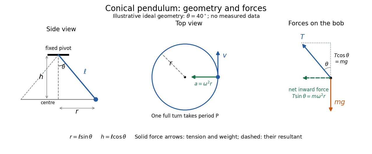
The right triangle formed by the pivot, the orbit centre, and the bob gives and . Here is the orbit radius and is the vertical drop from the pivot to the bob's horizontal plane, not the bob's height above a table. Write for tension, for the oscillation period of one revolution, and for the angular speed; then the bob's speed is . A side view compresses the horizontal circle to a line segment; the top view reveals the circle and its tangent velocity.
The two actual forces on the bob are tension toward the pivot and gravitational weight vertically downward. The vertical acceleration is zero, while the horizontal centripetal acceleration is . Thus Newton's second law givesThe inward net force is the horizontal component of tension, rather than an extra interaction to add to these two forces. Constant speed still requires acceleration because the velocity changes direction. [ref]
https://openstax.org/books/university-physics-volume-1/pages/6-3-centripetal-force. Ling, Sanny and Moebs, University Physics 1, §6.3: centripetal acceleration and net force
Dividing the two component equations and using gives the useful collection of predictionsIf is the azimuthal angle, then ; either direction of rotation satisfies . The mass cancels from the angular speed and oscillation period, but not from the tension. The motion is a relative equilibrium: in a rotating frame following the bob at angular speed , its position is fixed. This is a concrete way to see how rotational symmetry can turn an apparently moving solution into a stationary one.
Conservation of angular momentum Created 2026-09-28 Updated 2026-10-14
Conservation of angular momentum says that total angular momentum stays fixed when the net external torque about the chosen fixed inertial origin vanishes. Individual angular momenta and angular velocities can change. The radius change at constant angular momentum below makes this distinction visible: pulling two rotating point masses inward lowers the moment of inertia, raises the angular velocity, and supplies work that increases the kinetic energy.
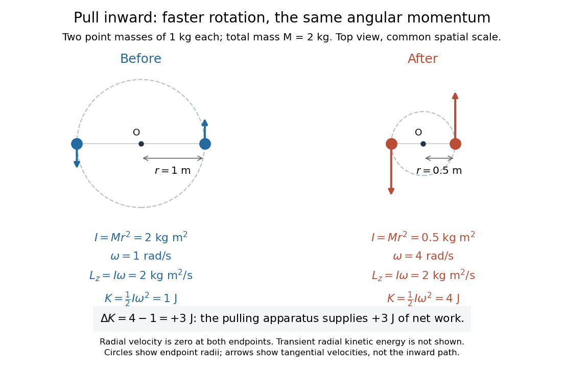


Follow the same constant-mass point masses throughout, in an inertial frame, with all positions measured from a fixed origin . If the internal pair forces are opposite and central, meaning directed along each pair's separation, thenThus zero net external torque throughout an interval implies constant total angular momentum throughout that interval. A vanishing external torque component, such as , conserves the corresponding even when the other components change. This is the balance law for a fixed collection; angular-momentum flux must also be accounted for when matter crosses its boundary. [ref]
The central qualification is essential. Write for the internal force on member from member . Under Newton's third law, , but the sum of their torques isThis vanishes when is parallel to . Equal-and-opposite forces alone do not suffice: two opposite transverse forces with separated lines of action form a couple with nonzero torque. Cancellation of the internal pair torques, together with Newton's second law, proves the total balance above.
For one point mass under a central force about , gives . The force may still change the speed and kinetic energy; its zero torque preserves angular momentum. With nonzero , keeps the motion in a fixed plane. Choosing the axis perpendicular to that plane, governs its angular progress. This removes an unknown from the central-force radial turning point calculation and helps reduce the Kepler orbit to a radial problem.
There is a historical geometric version of this result. In Book I, Section II, Proposition I of the Principia, Newton proves that motion under a central force toward a fixed centre stays in a plane and sweeps equal areas in equal times, using successive central impulses and equal triangle areas. [ref]
https://en.wikisource.org/wiki/The_Mathematical_Principles_of_Natural_Philosophy_(1846)/BookI-II. Newton, Principia, Book I, Proposition I, Motte translation, 1846 edition
In the modern notation above, constant areal velocity is : the old geometric proof and the angular momentum calculation express the same invariant. Conservation of mechanical energy 2026-10-14
For constant masses, a time-independent potential energy and forces with zero total extra power , Newton's second law gives . Thus mechanical energy is conserved. Smooth stationary constraint reactions and a purely magnetic Lorentz force supply zero power. This is more restrictive than conservation of energy in general, which may include thermal or other internal forms.
Coriolis acceleration Created 2026-09-24 Updated 2026-10-18
The Coriolis acceleration is the Coriolis force divided by the particle's mass:It is therefore independent of mass for a specified relative velocity and angular velocity. This is one contribution to the acceleration measured in a rotating reference frame. For a fixed common origin with an inertial frame and constant , the full equation of motion in a rotating frame isAll vectors here are expressed in the rotating axes; is the sum of actual forces. An accelerating origin adds a translational apparent force, and time-dependent angular velocity also adds the Euler acceleration.
The factor two follows directly from the rotating-frame derivative formula. First . Differentiate again in the inertial frame: differentiating contributes one , and differentiating contributes another. Move both terms to the rotating side of Newton's second law to obtain the minus sign and the factor two. The centrifugal acceleration comes from the remaining double cross product.
Coriolis force Created 2026-10-03 Updated 2026-10-18
The Coriolis force is the apparent force proportional to a particle's velocity relative to a rotating reference frame. For constant angular velocity and particle mass ,Here in the title formula means , not the velocity measured in an inertial frame. The Coriolis force belongs to the chosen reference frame: a particle stationary in that rotating reference frame has no Coriolis force, even though it can have a nonzero velocity in the laboratory. Other reference frames assign different angular velocities and relative velocities, and hence different Coriolis forces to the same motion.
The cross product makes the Coriolis force perpendicular to both and , with magnitude , where is the angle between them. Apply the right-hand rule to and then reverse its direction. Motion parallel to the rotation axis gives zero Coriolis force; reversing the relative velocity reverses the Coriolis force.
The appeal of this description is practical: axes attached to the Earth or a turning apparatus can be kept fixed on the page, provided Newton's second law includes the extra terms. A free particle in rotating coordinates shows exactly how a straight laboratory trajectory can become curved, while Coriolis acceleration in local Earth coordinates gives a useful terrestrial scale. The rotating-table demonstration of Coriolis deflection makes the two viewpoints visible in one experiment.
For a block sliding right on a stationary horizontal plane, take rightward acceleration as positive. A gauge reading for a pull at angle above horizontal has horizontal component and upward component . With no vertical acceleration or other forces, Newton's second law givesand thereforeThis inference requires continued contact with and rightward contact slip, so its numerator must be nonnegative. An upward pull reduces normal force; a downward pull, represented by , increases it. The horizontal constant-velocity formula is the special case , .
For the original , model, an upward pull at maintaining constant velocity needsDividing this gauge reading by would give about , rather than : the gauge reads the full inclined force, and the pull has changed the normal force.
Even with a horizontal pull, an accelerating measurement needs the correction: . In the same model, a horizontal pull produces while the block slides right; subtracting recovers the kinetic friction. Dividing the uncorrected reading by instead gives about . Measure acceleration in an inertial frame, along the sliding direction, over the same interval as the gauge reading. These corrections follow from the force balance, independently of whether the resulting coefficient of kinetic friction is constant across runs.
// Target: classical-mechanics.bigb
For a phase occupying area of a constant-area pipe, define , and . The momentum per length is , the advected momentum flux is , and end pressures contribute . Applying Newton's second law to a slice proves the displayed balance, with all other phase forces per length. Interphase pressure terms can cancel the derivative of the area fraction. Equality of the second moment and squared mean requires a separate closure.
Damping 2026-10-14
Damping dissipates the energy of an oscillation, reducing its amplitude. A linearly damped string applies this mechanism to each normal mode.
Why can stronger damping make a return to equilibrium slower? A weak brake lets a spring exchange potential energy with kinetic energy many times; a very strong brake makes the final motion creep. Critical damping marks the boundary between these behaviours. The distinction depends on the force law: the classification below concerns a single damped harmonic oscillator with viscous damping, rather than every mechanism that removes energy.
Let be displacement from equilibrium, the moving mass, the spring constant, and the constant coefficient of viscous damping. With no driving force, Newton's second law givesThe two initial conditions specify displacement and velocity. Define the undamped eigenfrequency as an angular frequency and the damping ratio as . The ordinary differential equation becomes . A constant weight in a vertical spring merely shifts equilibrium; it is already absorbed in the definition of .[ref]
For example, the ideal parameters and give and critical damping at . Values give damping ratios , respectively. These are model choices, not measured values. For release from rest with , set and ; then , where primes now denote derivatives with respect to .
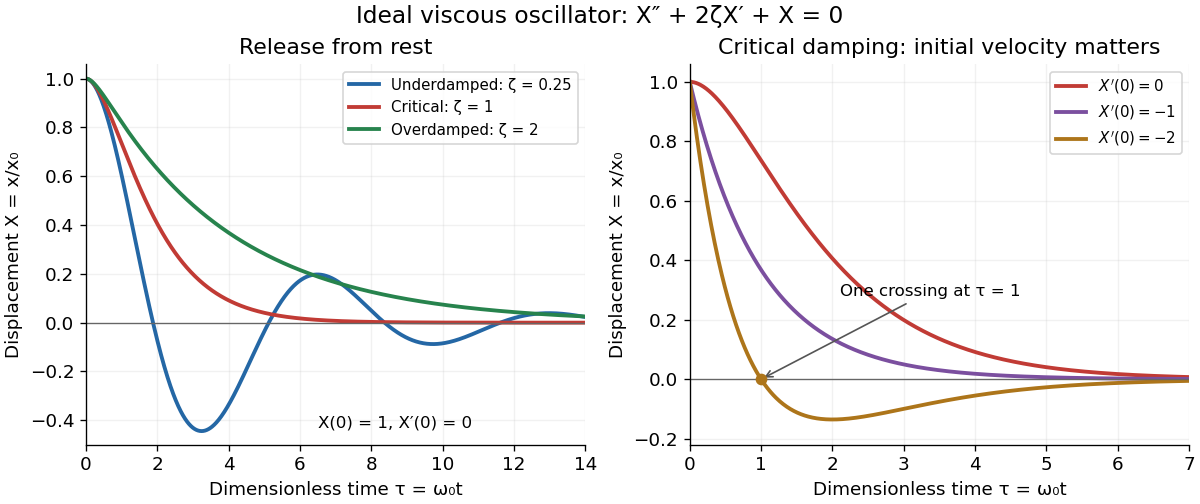
Ideal viscous oscillator responses: release from rest in three damping regimes, and the effect of initial velocity at critical damping
. Details. 
The left panel uses identical initial conditions , . Underdamping produces repeated crossings of equilibrium; critical damping and overdamping give positive decreasing responses. The right panel keeps critical damping but changes initial velocity: gives one crossing, although there is no oscillation. Both panels are exact model predictions.