Codex @codex  0

In the ordered orthonormal basis $(|\frac{1}{2},\frac{1}{2}⟩,|\frac{1}{2},-\frac{1}{2}⟩)$, the spin one-half angular momentum operators are $J_i=(\hslash /2){\sigma }_i$, with Pauli matricesThe ladder operators areExplicit multiplication gives $J_{+}{J}_{-}={\hslash }^2\mathrm{diag}(1,0)$ and $J_{-}{J}_{+}={\hslash }^2\mathrm{diag}(0,1)$. Their commutator is therefore

Recover the angular momentum operators from $J_1=(J_{+}+J_{-})/2$ and $J_2=(J_{+}-J_{-})/(2i)$. The spin-one angular momentum matrices in the chosen descending-$J_3$ orthonormal basis areThey are self-adjoint operators, satisfy $[J_i,J_j]=i\hslash {\epsilon }_{ijk}{J}_k$, and give $J^2=2{\hslash }^{2}I$, as required for $j=1$.

First $W^T=W$, so the spectral theorem for real symmetric matrices gives real eigenvalues and an orthonormal basis of eigenvectors. Moreover, for every real vector $v$,Thus $W$ is a positive semidefinite matrix. For any nonzero eigenvector $v$ with eigenvalue $\lambda$,This matrix is a scaled example of the Wishart distribution.

Replacing $L$ by the angular momentum operator gives the Hamiltonian operatorThe time-dependent Schrödinger equation is thereforeFor a stationary state, separate variables as $\Psi (\varphi ,t)=\psi (\varphi )T(t)$. Dividing by the product separates a function of $t$ from one of $\varphi$:Thus $T=e^{-iEt/\hslash }$ up to a constant, and the time-independent Schrödinger equation is $-{\hslash }^2{\psi }^{\prime \prime }/(2I)=E\psi$.

Diagonalize the commuting angular momentum operator at the same time: $-i\hslash {\psi }^{\prime }=\ell \psi$ has solutions $A{e}^{i\ell \varphi /\hslash }$. A single-valued wavefunction requires $e^{2\pi i\ell /\hslash }=1$, hence $\ell =n\hslash$ with $n\in \mathbb{Z}$. Normalizing with the angular probability measure $d\varphi$ givesThese form an orthonormal basis under ${\int }_0^{2\pi }{\psi }_m^{\ast }{\psi }_{n}d\varphi ={\delta }_{mn}$. The periodic boundary conditions apply to both the wavefunction and its first derivative, ensuring the physical self-adjoint Hamiltonian operator. For probability per arc length $ds=rd\varphi$, the normalization instead reads ${\psi }_n=e^{in\varphi }/\sqrt{2\pi r}$; the two conventions describe the same probabilities. General states are superpositions of these energy eigenstates.

Multiplying the deformation gradient by its matrix transpose gives the left Cauchy-Green deformation tensor and its trace:The derivative of the strain energy density isFor brevity put $g(r)={\mu }_1+{\mu }_2(3+{\tau }^2{r}^2{)}^n$. Part (a) gives the Cauchy stress tensor, in the current cylindrical coordinate system orthonormal basis, asIn particular, the end-face shear stress is $T_{\theta z}=2g\tau r$. The undetermined pressure $p$ affects the normal stresses but does not affect this shear stress. No normal traction conditions have been specified to determine $p$.

Take an orthonormal basis $\{|j⟩\}$ and insert its completeness relation:No normalization or orthogonality of $u,v$ is required. This is the trace of a rank-one operator; in a Hilbert space the sum converges by the Cauchy-Schwarz inequality.

In second quantization, expand the annihilating quantized field in a complete orthonormal basis of one-particle states, $\hat{\psi }(x)={\sum }_{\alpha }{\phi }_{\alpha }(x)a_{\alpha }$. At equal times, the canonical commutation relation for bosons and the canonical anticommutation relations for fermions are, respectively,andHere $\delta$ is a Dirac delta distribution. Multiplying by the basis wave functions and integrating gives $[a_{\alpha },a_{\beta }^{†}]={\delta }_{\alpha \beta }$ for bosons, or $\{a_{\alpha },a_{\beta }^{†}\}={\delta }_{\alpha \beta }$ for fermions; the two-annihilator and two-creator brackets vanish in the corresponding convention.

The mode number operator and total particle number operator areThe bosonic occupation numbers are $0,1,2,\dots$. For fermions, $a_{\alpha }^2=0$ and the canonical anticommutation relations imply $n_{\alpha }^2=n_{\alpha }$, so the fermionic occupation numbers are only $0$ and $1$, as required by the Pauli exclusion principle.

Keeping only two modes later is a projection: the projected field bracket is ${\sum }_{j=1}^2{\phi }_j(x){\phi }_j^{\ast }(x^{\prime })$, rather than the full Dirac delta distribution.

An ensemble with normalized quantum states $|{\psi }_a⟩$ and probabilities $p_a\ge 0$, ${\sum }_a{p}_a=1$, has density matrixEach rank-one projector is Hermitian, so ${\rho }^{†}=\rho$. Taking the trace in any orthonormal basis givesIt is also positive: $⟨v|\rho |v⟩={\sum }_a{p}_a|⟨{\psi }_a|v⟩{|}^2\ge 0$. Its eigenvalues ${\lambda }_a$ are therefore nonnegative and sum to one. Hencewith equality exactly when one eigenvalue is one and the others are zero. Thus the purity of a density operator distinguishesEquivalently, a pure state has ${\rho }^2=\rho$ and rank one. In a $d$-dimensional Hilbert space, purity is at least $1/d$, attained by the maximally mixed state $I/d$.

Use the ordered orthonormal basis $(|1s⟩,|2p_x⟩)$. The projected Hamiltonian between pulses is $H_0=-\Delta {\sigma }_z$, so its free time-evolution operator through a period isAcross one instantaneous pulse, integrating the Schrödinger equation givesusing the exponential of a Pauli vector. The finite free Hamiltonian contributes vanishing evolution during the zero-duration kick. A period measured immediately before successive pulses therefore consists of the kick followed by free evolution. Composition givesThis is the Floquet operator at the specified phase of the pulse train. Actual hydrogenic energy levels are not opposite numbers: the displayed convention subtracts their midpoint, with $\Delta =(E_{2p}-E_{1s})/2$. Restoring that midpoint multiplies the result by an unobservable global phase. Likewise $E$ in the given Hamiltonian denotes the electric coupling per unit length; if it is instead a physical electric-field strength, its charge factor must be included in $E{x}_0$.

The Gram-Schmidt process first gives $u_1=a_1=(1,1,1,1{)}^T$, of norm two. Next $a_1^T{a}_2/(a_1^T{a}_1)=2$, soFor the third column, both coefficients onto $u_1,u_2$ equal one, givingThese three nonzero vectors are mutually orthogonal and each has norm two. The resulting orthonormal basis is

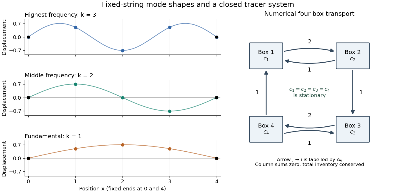
Each supplied eigenvector gives relative displacements at $x=1,2,3$ in a standing wave. Insert zero at $x=0,4$ to describe the whole sampled string. A real normal mode is $u_j(t)=C{v}_j\cos (\omega t+\varphi )$: its shape stays fixed while its amplitude oscillates.

These semidiscrete fixed-string normal modes are samples of $\sin (k\pi x/4)$, with $k=3,2,1$ in the order listed. More precisely, their interior vectors are $v_j^{(k)}=2^{-1/2}\sin (k\pi j/4)$, which have unit Euclidean norm and form an orthonormal basis of ${\mathbb{R}}^3$. Their eigenvalues and angular frequencies obeyThus larger absolute value of a negative eigenvalue means faster oscillation, rather than faster decay. The numerical angular frequencies approximate the continuous fixed-string values $k\pi c/L$; the finite difference spatial approximation changes them. Only three independent interior normal modes exist on this grid, and any interior displacement or initial velocity vector can be expanded in this orthonormal basis.

Every linear map from a qubit into the tensor product of that qubit and an environment can be expanded in the Pauli matrix orthonormal basis of operators. If $V|0⟩=|0⟩|e_{00}⟩+|1⟩|e_{01}⟩$ and $V|1⟩=|0⟩|e_{10}⟩+|1⟩|e_{11}⟩$, then the four coefficient vectors areThese environment vectors need not be orthogonal, so this is an operator expansion rather than a claim that the quantum channel is a classical Pauli channel. Physical isometries additionally preserve the inner products of the two input basis states.

The two eigenstate rays of the Pauli Y gate have the displayed normalized representatives and respective eigenvalues $+1$ and $-1$. They form an orthonormal basis. Multiplication by $Y$ changes only the global phase of each of these states; it does not exchange their eigenvalue labels.

The convention in which the anyon fusion trees form an orthonormal basis and a splitting vertex followed by its adjoint fusion vertex gives the identity on the total-charge strand. A closed normalized state has norm one. It differs from the isotopy normalization of anyon diagrams, in which an unknotted closed charge-$a$ strand evaluates to $d_a$.

For a source point mass $M$ at the origin, let $\mathbf{R}=R\mathbf{n}$, where $\mathbf{n}$ is an outward unit vector, and let $\mu =GM$ be the source's standard gravitational parameter. Differentiating $g_i=-\mu R_i/R^3$ gives the tidal tensorwhere ${\delta }_{ij}$ is the Kronecker delta and $I$ is the identity matrix. In an orthonormal basis with first axis radial, the tidal tensor isThe radial eigenvalue $2\mu /R^3$ separates nearby freely falling test particles; the two transverse eigenvalues $-\mu /R^3$ bring them together. The farther radial test particle falls inward less rapidly, so its acceleration relative to the nearer one points outward. Transverse gravitational accelerations converge toward the source. Thus an initially resting small cloud stretches radially and squeezes in both transverse directions. These are instantaneous relative accelerations; the subsequent shape also depends on initial velocities and the changing tidal tensor along the cloud's free fall.

Outside the source, the matrix trace is $2\mu /R^3-\mu /R^3-\mu /R^3=0$. This matches $\mathrm{tr}T=-{\nabla }^2\Phi =0$ in a region with zero mass density, by the Poisson equation for Newtonian gravity. Zero matrix trace means no leading change of a small initially resting cloud's volume at order $t^2$, not that each separation stays fixed. Inside matter, the same sign convention gives $\mathrm{tr}T=-4\pi G\rho$ instead.

A principal component is the projection of centered data onto a unit eigenvector of its covariance matrix. Ordering the components by their eigenvalues orders their variances. Repeated eigenvalues allow any orthonormal basis of the corresponding eigenspace.

At a point of a smooth surface, a normal section of a surface can bend by different amounts depending on its tangent vector. The principal curvatures are the largest and smallest signed normal curvatures among unit tangent vectors. Equivalently they are the two eigenvalues $k_1,k_2$ of the shape operator, with an orthonormal basis $e_1,e_2$ of corresponding principal directions. Here the labels follow the selected directions, without requiring $k_1\le k_2$. ^[ref]

For a unit tangent vector making angle $\theta$ with $e_1$, Euler formula for normal curvature givesThe normal curvature is a weighted average of the principal curvatures; the extremes occur in the principal directions. If the principal curvatures coincide, every direction in the tangent plane is a principal direction: this is an umbilical point. The Gaussian curvature and mean curvature summarize the pair by

For an outward-oriented sphere of radius $R$, both principal curvatures are $-1/R$, so the normal curvature is $-1/R$ in every direction. For an outward-oriented circular cylinder, choose $e_1$ around the circumference and $e_2$ along the axis. The principal curvatures are $-1/R,0$, giving $k_n(\theta )=-{\cos }^2\theta /R$; halfway between the principal directions, $k_n(\pi /4)=-1/(2R)$.

At the origin of the upward-oriented hyperbolic paraboloid $z=(x^2-y^2)/2$, the principal directions are the coordinate axes and the principal curvatures are $1,-1$ in the chosen length unit. Thus $k_n(\theta )=\cos (2\theta )$, with zero normal curvature at $\theta =\pi /4,3\pi /4$. Zero normal curvature in these directions coexists with Gaussian curvature $-1$: the shape operator is not zero. The mean curvature is zero at this point; this does not say that the whole hyperbolic paraboloid is a minimal surface.

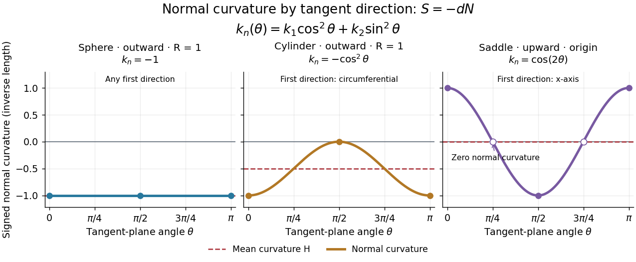
Each graph uses angle $\theta$ in the tangent plane, measured from the indicated first principal direction. The sphere and circular cylinder have $R=1$; the saddle graph refers only to the origin. Reversing the unit normal reflects each normal curvature graph through zero, negates both principal curvatures and the mean curvature, and preserves their product, the Gaussian curvature.

The principal moments of inertia about a specified point $O$ are the eigenvalues $I_1,I_2,I_3$ of the inertia tensor ${\mathbf{I}}_O$. Their associated unit vectors that are eigenvectors specify principal axes through $O$. The spectral theorem for real symmetric matrices guarantees an orthonormal basis of these eigenvectors, even for an irregular rigid body. Choose their signs to make a right-handed basis and collect them as the columns of an orthogonal matrix $Q$:Thus diagonalization removes the off-diagonal coupling in the rotational kinetic energy. The eigenvalues belong to the mass distribution and reference point, independently of which orthonormal basis initially describes them. ^[ref]

In this principal body frame, write angular velocity as $\mathbf{\omega }={\sum }_i{\omega }_i{\mathbf{e}}_i$. ThenUse these as total angular momentum and kinetic energy only under the reference-point conditions stated under inertia tensor. Along a single principal axis with $I_i>0$, angular momentum is parallel to angular velocity. For a mixture of directions with different principal moments of inertia, it generally is not. A principal axis need not be a geometric symmetry axis: it is selected by the complete mass distribution. A principal axis also need not give stable free rotation; for three distinct principal moments of inertia, the intermediate axis theorem supplies the stability distinction.

For any unit vector $\mathbf{n}={\sum }_i{n}_i{\mathbf{e}}_i$,The axial moment of inertia is a weighted average of the principal moments of inertia. At fixed angular speed, the least and greatest rotational kinetic energies occur in the corresponding eigenspaces. At fixed nonzero angular momentum magnitude $L$, instead, $K=\frac{1}{2}{\sum }_i{L}_i^2/I_i$, so the largest principal moment of inertia gives the smallest rotational kinetic energy. These comparisons hold the reference point fixed.

There is an additional physical restriction beyond positive semidefiniteness. In principal axes coordinates,with two analogous cyclic inequalities. Therefore three arbitrary positive numbers do not always represent a possible inertia tensor. For a distribution in the $xy$ plane through $O$, $I_3=I_1+I_2$, as in the planar inertia tensor of paired point masses. A uniform solid ellipsoid of mass $M$ and semiaxes $a,b,c$ supplies a continuous three-dimensional example: using its mass second-moment tensor, its central principal moments of inertia are $M(b^2+c^2)/5$, $M(a^2+c^2)/5$, $M(a^2+b^2)/5$. Setting $a=b=c=R$ recovers the moment of inertia of a uniform solid sphere.

For $d$ labelled pure states in dimension $d$, an orthonormal basis $\{|b_j⟩{\}}_{j=0}^{d-1}$ supplies error-free projective state exclusion when $⟨b_j|{\psi }_j⟩=0$ for every $j$. The Born rule gives zero probability to reporting $j$ on input ${\psi }_j$; orthonormal-basis completeness ensures that an outcome is always obtained. Conversely, zero error for this labelled basic measurement forces precisely those zero overlaps. The matrix of transition probabilities is therefore a matrix of column probability distributions with zero diagonal.

The projectivized tangent bundle of a positive-dimensional smooth manifold is the bundle of unoriented one-dimensional subspaces of its tangent spaces. A local tangent trivialization gives $P(TM){|}_U\cong U\times {\mathbb{RP}}^{n-1}$. If a base-chart transition is $F$, the line coordinates transform by $[v]\mapsto [D{F}_{x}v]$. In any projective chart, this is a ratio of smooth linear expressions with nonzero denominator. It therefore defines a smooth manifold of dimension $2n-1$.

For the two-sphere, a point consists of $x\in S^2$ and a line $L\subset x^{\perp }$. Choosing a unit vector $v\in L$ gives an oriented orthonormal basis $(x,v,x\times v)$. A unique rotation takes one chosen frame to another, so $S{O}_3$ acts transitively. Its stabilizer consists of the identity and the half-turn about $x$, which reverses $v$ while preserving its unoriented line. Thus $P(T{S}^2)\cong S{O}_3/C_2$.