Source paper: public source PDF, pages 79–86. The cover identifies the examination as 2021 despite the archive filename. Solutions cover all three options. The damaged source diagram leaves the numerical results in S02 1(b) and 1(d) incomplete.
The apparent singularity at zero cancels: the Taylor series of the sine givesThus zero is a removable singularity, with extension . At , the other terms are holomorphic, whereas has a simple pole. ThereforeThere are no other finite singularities. If “all” includes the point at infinity on the Riemann sphere, it is an essential singularity: has infinitely many negative powers in its Laurent series at .
The geometric series for converges for , while the cancelled sine terms have an everywhere convergent Taylor series. Hence the requested Laurent series has no negative powers:For example,The extension through zero also makes this a Taylor series. The pole at fixes its radius of convergence at two.
Assume positive, counterclockwise orientation of a contour. Factor the polynomial denominator asOnly lie inside the unit circle. These are simple poles. Writing the denominator as , their residues areThe residue theorem therefore givesReversing orientation of a contour changes the sign.
Parametrize the positively oriented unit circle by . Then andConsequently the contour integral already evaluated satisfies
Let be holomorphic on a neighbourhood of a positively oriented, piecewise smooth simple closed curve and its interior except at finitely many isolated singularities strictly inside. The residue theorem statesThe residue is the coefficient of in the local Laurent series. No singularity may lie on the contour. For more general closed contours, each residue is multiplied by the corresponding winding number.
The poles are the four roots of . The upper half-plane contains and , both enclosed when . At a simple pole ,The sum of the two residues isThe residue theorem, with the real segment traversed from to and the upper arc from to , yields
On the upper semicircular contour, and the reverse triangle inequality gives . Its arc length is , so the estimation lemma givesThe arc is open, so an ordinary integral sign is appropriate even though the source uses a closed-integral symbol there. Subtracting the vanishing arc contribution from the closed contour integral gives the real-line improper integral . Its integrand is an even function, and its tail is , ensuring convergence. Thus
Use the principal complex square root, with . For , the local expansion on this holomorphic branch isThe fractional power prevents a single-valued Laurent series in a punctured disc. In particular, zero is a branch point, not an isolated singularity classified as a pole. Merely observing that on the slit plane would not establish a simple pole: does not extend as a holomorphic function through a whole disc around zero.
The negative real half-line is a chosen branch cut. Its upper and lower boundary values differ because and for . Continuation once around zero changes the sign of the complex square root, and hence changes in general. Other branch cuts are possible; this one defines the principal holomorphic branch.
Excise a small disc about zero and a thin slit along the negative real axis, using the orientations shown in the source: upwards, towards zero above the slit, clockwise around zero, and away from zero below the slit. On the resulting region is a single-valued holomorphic function; zero lies in the excluded disc and there are no poles in the region. Cauchy's integral theorem givesHere the paths on the cut mean limiting paths from its two sides. Apply Cauchy's integral theorem before taking those limits, when the entire contour lies inside the slit domain.
For , the upper and lower boundary values on the branch cut areWrite for the outer endpoint distance on the cut. The upper path runs from to , while the lower path runs back from to ; in both cases . ThereforeandThe source's limits zero and infinity require and ; they are not an exact identity on a finite contour. For a concrete counterexample take and : the finite real integral is at most , whereas the full-range integral is , as evaluated in the next part. Near zero the combined integrand is , so the combined improper integral converges, although the individual cut integrals have logarithmic divergences. At infinity the factor ensures convergence. Consequently
On the small clockwise contour , decreases from to . Uniformly on that arc, , and henceThe large arcs also vanish. To make this precise for the displayed geometry, take them on the left semicircle , , split at the cut. On the principal holomorphic branch, , , and . The estimation lemma givesFor the last bound, symmetry and on imply that the angular integral is at most . The exact choice of large arcs does not affect the limiting result. The vertical improper integral converges absolutely because decays as .
Taking limits in the closed contour integral now yields , where . ThusAs an optional explicit evaluation, put and define . Differentiation under the integral sign and the Gaussian integral give and . Therefore and in terms of the error function and complementary error function.
The astronomical magnitude convention is , with both fluxes measured through the same photometric passband. A five-unit magnitude difference therefore corresponds toThe brighter endpoint has one hundred times the visual flux of the fainter endpoint. Absolute fluxes require a magnitude zero point, which is not given.
TODO: numerical endpoints require the unreadable source diagram. Let and be the maximum and minimum main sequence visual luminosities, in units of the Sun's visual luminosity. At a distance , the inverse-square law and the magnitude difference relation giveThus, using ,At the naked-eye detection threshold , the greatest distances for the intrinsically brightest and faintest main sequence stars would respectively beThe historical endpoint is a brightness reference, not the visibility threshold: if that endpoint were intended instead, the corresponding coefficient would be rather than .
The source Hertzsprung-Russell diagram has lost the stellar loci and luminosity scale except for a surviving top tick; neither endpoint can be read reliably. If its scale was bolometric luminosity rather than visual luminosity, bolometric corrections would also be needed, especially for very hot and very cool stars. Equating the two luminosity ratios would then be an explicitly approximate assumption. These missing data are not replaced by invented endpoint values. Interstellar extinction is neglected in the displayed distance relation.
For spherical hydrostatic equilibrium, the stellar structure equations includeEliminate to obtain . Since through the interior, integration givesWith negligible surface pressure, this provesThis is a conservative lower bound; concentrating mass near the centre increases the required pressure.
For the temperature inference assume predominantly ideal gas support, a nearly fully ionized hydrogen–helium mixture with mean molecular weight , and the hottest region at the centre. A rigorous scale estimate follows from the stellar virial theorem, rather than substituting the mean mass density for the unknown central mass density. With negligible surface pressure,The ideal gas law gives . The mass-weighted mean temperature consequently obeysThis establishes several million kelvin under the stated physical assumptions. The central pressure inequality alone does not give a central temperature bound without an equation of state and information about mass density or an integrated argument.
TODO: the plotted location of Procyon B is missing from the damaged source diagram. The Stefan–Boltzmann law would determine the stellar radius from its effective temperature and bolometric luminosity:A visual luminosity alone must first be converted with the appropriate bolometric correction. Procyon B is a white dwarf, so its small stellar radius and hot surface place it below the main sequence, rather than among giant stars or supergiants. This classification does not supply the missing numerical coordinates. A source-based numerical stellar radius cannot be claimed from the surviving image.[ref]
Hubble Space Telescope Astrometry of the Procyon System. Abstract: the companion Procyon B is identified as a DQZ white dwarf
The intact source figure gives orbital period , stellar radial velocity semiamplitude , and orbital eccentricity . A planetary exoplanet transit implies a nearly edge-on orbit, so . Adopt a solar mass for the Solar-type star and initially neglect the companion's mass relative to it.
For a circular solution of the two-body problem, the star's distance from the centre of mass is , and the measured semiamplitude is . Kepler's third law givesHenceThe inferred binary mass ratio is only , validating the approximation. Since , the star–planet separation is constant and equals the orbital semimajor axis. Without the exoplanet transit, Doppler spectroscopy would generally give only a minimum companion mass through .
Assume uniform reradiation over the planetary surface, unit thermal emissivity, and zero Bond albedo. The planet absorbs over its projected disc and emits over its full sphere. Radiative equilibrium and the Stefan–Boltzmann law giveUsing the liquid-water range as the crude thermal criterion givesFor nonzero Bond albedo , both radii acquire the factor . For example gives approximately to . An airless planet need not have uniform surface temperature; inefficient heat redistribution makes the dayside hotter and the nightside colder, so a single equilibrium temperature is an averaging approximation.
This simple habitable zone contains the Earth's orbit under the zero-albedo assumption, but also contains Venus's orbit, although its greenhouse effect produces an uninhabitably hot surface. Mars lies beyond the calculated outer boundary. These comparisons show the usefulness of the orbital scale and the limitations of a temperature-only criterion. The stipulated airless model also omits the atmospheric pressure needed for stable surface liquid water: this is an effective thermal window, not a sufficient habitability condition.
Transit photometry. A planet crossing the stellar disc produces a periodic reduction in flux, approximately for a small, dark planet away from the limb. The orbital period and stellar radius allow an inferred planetary radius, but not its mass by this method alone. The geometric geometric transit probability is roughly for a circular orbit, so the method strongly favours close orbits and large planets. Small signals compete with instrumental noise and stellar activity; eclipsing stellar binaries and blended sources can mimic a planetary exoplanet transit, and long orbital periods require long observing baselines.
Doppler spectroscopy. Periodic shifts of stellar spectral lines reveal the stellar radial velocity caused by motion around the centre of mass. For a light companion, , favouring massive, short-period companions and low-mass host stars. Unknown orbital inclination gives a minimum mass; stellar activity, line broadening, and instrumental calibration limit precision. Long orbital periods require years of measurements.
Direct imaging. Spatially resolved reflected light or thermal emission separates a planet from its host. The large star–planet brightness contrast and small angular separation demand starlight suppression and precise correction of optical aberrations. The method favours wide orbits around nearby stars, and young, hot, massive planets with stronger thermal emission. Translating brightness to mass depends on planetary cooling models and age; it is difficult to image an Earth analogue close to a bright star.
For the estimate implied by the supplied Hubble constant, use the low-redshift Hubble law . ThenWith radians, inversion of the Einstein angular radius relation givesThe corresponding projected Einstein radius is .
This is the projected enclosed mass of the galaxy cluster, including all matter, not just its stars. Strictly, the gravitational lensing formula uses angular diameter distances, and at the low-redshift approximation is only an estimate. An exact value requires a specified cosmological expansion history and a consistent lens-to-source angular diameter distance; it cannot be determined from alone. The later estimates use the same distance approximation consistently.
Assume virial equilibrium, structurally homologous early-type galaxies, a fixed relation between the measured central velocity dispersion and the global random stellar motions, and a constant total mass-to-light ratio . The virial theorem gives , where the dimensionless structure factor is common to the sample. With denoting mean linear surface brightness inside the effective radius, . ThusThe usual observed fundamental plane of elliptical galaxies has a tilt relative to these exponents because mass-to-light ratio varies with stellar population, chemical composition, and dark matter fraction; structural and dynamical nonhomology can also change .
Printed convention. The source places the logarithm of a value expressed in in the empirical fit. This differs from the usual logarithm of linear surface brightness. If is the quoted magnitude surface brightness,A coefficient on therefore becomes on , with an adjusted intercept; it does not become . For a concrete distinction, changing from 20 to 25 decreases linear surface brightness by a factor 100, so the linear-intensity fit changes by , whereas the literal printed logarithm changes it by .
The following part evaluates the printed numerical fit literally and labels that convention. If the fit was intended for linear surface brightness, its calibration must be specified; a conditional result for using the same coefficients with linear units is also given. No equality between these two conventions is assumed.
Evaluate the source's printed logarithm using the numerical magnitude value 21.0, with base-ten logarithms:This is the literal printed-fit convention identified above. Convert the mean visual surface brightness to a linear luminosity per projected area. At 10 parsecs, one square arcsecond subtends . The definition of absolute magnitude consequently givesThe constant is the conversion between the angular and physical projected area. Since the effective radius encloses half the total luminosity,For the stipulated stellar population of Solar-type stars, approximate the stellar mass-to-light ratio by . Summing 100 such galaxies then givesThis assumes negligible interstellar extinction and that the supplied surface brightness is an intrinsic or already corrected value; an observed cosmological surface brightness requires additional dimming and passband corrections before this conversion.
For comparison only, if the empirical coefficients and intercept were instead meant for , substituting in that fit would give , , and . Those are conditional alternative results, not an unannounced correction of the printed units.
The gravitational lensing mass includes dark matter, hot intracluster gas, stars, and any other material in the projected aperture. Most is not stellar: in the literal convention above the stellar fraction is only .
Assume the cluster shares the cosmic cosmic baryon fraction, , and compare the same aperture for all components. ThenNeglecting stars entirely would give . Thus the assumed hot gas dominates the baryonic matter, and the remainder is dark matter. The budget is consistent: stars are about of the inferred baryonic matter, and all components sum to .
For a thermal scale, take gas extent and mean particle mass with for ionized gas. A simple spherical virial theorem estimate with gas binding energy and thermal kinetic energy givesThis is the scale of a very hot, massive X-ray emitting galaxy cluster. The numerical prefactor depends on the radial mass density profile, gas distribution and boundary pressure; for example an isothermal-sphere estimate gives about . Moreover is a projected aperture mass at , whereas the estimate needs a spherical enclosed mass at ; the given data do not determine that conversion. The quoted temperature is therefore an order-of-magnitude estimate, not a uniquely measured value. Nor do the data determine the total gas mass outside the Einstein ring without a profile. The gas budget above pertains to the matched aperture under the cosmic-fraction assumption.
A blackbody absorbs all incident electromagnetic radiation, at every frequency, direction and polarization: its absorptivity is one. In thermal equilibrium, Kirchhoff's law of thermal radiation makes its emissivity one as well. Its emitted spectrum depends only on its absolute temperature, through Planck's law, rather than on the material of its surface.
A small aperture in a large isothermal cavity approximates a blackbody because radiation entering it undergoes many reflections and is very unlikely to escape before absorption. The equilibrium radiation field is isotropic and unpolarized. The total emitted radiant exitance is by the Stefan–Boltzmann law; the peak of the wavelength spectrum shifts to shorter wavelengths as temperature increases according to Wien's displacement law. An ideal absorber can therefore glow brightly when hot: “black” describes absorption, not the absence of thermal emission.
Here is the Planck constant, is the radiation frequency, is the speed of light in vacuum, is the Boltzmann constant, and is the absolute temperature in kelvin. The quantity is spectral energy density per unit frequency, so is energy per unit volume in the interval , and is dimensionless.
Put . In the long-wavelength limit , the Taylor expansion in Planck's law gives the Rayleigh-Jeans law,This is the classical equipartition theorem result: each electromagnetic mode carries mean energy . Extending it to arbitrarily high frequency would make the total energy density diverge, the ultraviolet catastrophe.
In the short-wavelength limit , , giving the Wien approximation,Large photon energies are thermally suppressed, removing the classical high-frequency divergence.
If the requested “form” is expressed per unit wavelength, the change of variables includes its Jacobian determinant: . ThusSubstituting without the Jacobian determinant would give an incorrect spectral density.
Convert the skin temperature to . To locate the peak per unit wavelength in Planck's law, write and maximize . Its positive stationary point obeysThis gives Wien's displacement law, . Hencein the thermal infrared. A peak per unit frequency would occur at a different spectral position; this answer uses the conventional wavelength peak.
For an ideal blackbody surface completely surrounded by an isothermal environment, the Stefan–Boltzmann law gives emitted power and absorbed power . The net outward radiative heat transfer is thereforeThe gross emitted power is about , but about is absorbed back from the surroundings. The difference, rather than the emitted term alone, is the relevant energy loss.
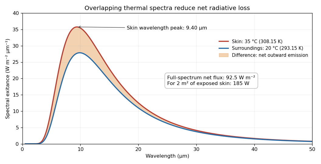
Skin and surroundings emit overlapping thermal spectra; their difference gives the net radiative loss
. Details. 
If the temperatures, exposed area, and surroundings remain fixed, the net radiated energy over one day isUsing the supplied conversion givesA dietary Calorie is one kilocalorie, so the result is about 3820 dietary Calories, rather than 3.82 million dietary Calories.
The estimate assumes the entire surface remains exposed at continuously. Clothing reduces direct exposure and presents a cooler outer emitting surface; the skin temperature also varies across the body and decreases in cooler surroundings through changes in blood flow. Body posture and nearby surfaces reduce the effective exchange area, while blankets and warm surrounding surfaces reduce net radiative heat transfer. These effects make the full-area, constant-temperature daily radiative estimate too large for ordinary clothed conditions.
The unit emissivity approximation is already fairly good for skin in the thermal infrared, so reducing emissivity alone is not the main correction. Also, convection, thermal conduction, and evaporation are additional channels of heat transfer; their existence does not subtract from the calculated radiative term. The computed number is a simplified radiative loss, not a complete metabolic energy budget.
In the photoelectric effect, incident light ejects electrons from a material when each absorbed photon supplies sufficient energy to overcome its work function . Conservation of energy gives the maximum emitted kinetic energy,At fixed frequency above threshold, increasing light intensity primarily increases the electron emission rate; it does not increase in the single-photon regime. Emission occurs without the long accumulation delay predicted for weak classical illumination.
Classical electromagnetism distributes incident energy continuously. By itself, that picture suggests that sufficiently intense or sufficiently long illumination could eject electrons at any frequency, and that emitted electron energies should increase with light intensity. It does not account for the observed threshold frequency and the linear dependence of on frequency with slope . Quantized photon absorption accounts for all three features.
The incident photon energy isSubtracting the work function gives . This is much less than the electron rest energy, so nonrelativistic kinetic energy is adequate:The magnitude of the retarding stopping potential satisfies , soThe collector must be negative relative to the emitting surface to retard the electrons; the quoted number is the magnitude. Contact-potential corrections are neglected.
The incident photon rate is . The stated quantum efficiency is , so the emitted electron rate is . If all emitted electrons are collected, the photocurrent magnitude isThe light power controls the number of events; the work function already determined the kinetic energy per emitted electron and should not be subtracted from the photon energy when counting incident photons. Incomplete collection would reduce the measured photocurrent below this value.
An electron accelerated from negligible initial kinetic energy through gains . The largest possible single photon energy in an X-ray tube is this entire kinetic energy, so the Duane-Hunt law givesThe massive anode can absorb the required recoil momentum with negligible recoil energy; most actual events produce lower-energy bremsstrahlung photons. The acceleration energy is valid without approximating the electron speed nonrelativistically.
Work in the initial rest frame of the free electron. If it absorbed a photon of positive energy , conservation of momentum would give the final electron momentum magnitude , while conservation of energy would give . But the final electron must obey the relativistic energy–momentum relation,Combining these statements giveswhich contradicts . ThusThe initial rest frame always exists for an electron, so this excludes the process in every inertial frame. Compton scattering is allowed because an outgoing photon carries additional energy and momentum. Absorption by an electron bound in matter is also possible because the rest of the system can share recoil.
For a particle on a circle, the tangential speed is , the moment of inertia is , and the angular momentum is . Hence its kinetic energy isThere is no potential energy variation along the circle in the stated model.
Replacing by the angular momentum operator gives the Hamiltonian operatorThe time-dependent Schrödinger equation is thereforeFor a stationary state, separate variables as . Dividing by the product separates a function of from one of :Thus up to a constant, and the time-independent Schrödinger equation is .
Diagonalize the commuting angular momentum operator at the same time: has solutions . A single-valued wavefunction requires , hence with . Normalizing with the angular probability measure givesThese form an orthonormal basis under . The periodic boundary conditions apply to both the wavefunction and its first derivative, ensuring the physical self-adjoint Hamiltonian operator. For probability per arc length , the normalization instead reads ; the two conventions describe the same probabilities. General states are superpositions of these energy eigenstates.
Applying the Hamiltonian operator to gives , and thereforeThe ground state has zero kinetic energy. Every positive energy level is of quantum degeneracy two, because and correspond to opposite angular momenta with equal squared magnitude.
The confinement scale suggests a tangential momentum scale and thus an excitation energy scale , consistent with the Heisenberg uncertainty principle. More precisely the de Broglie wavelength must fit an integer number of times around the circumference: , so . This explains both the dependence and the sequence.
One must not infer a nonzero ground-state energy by applying naively. Angle is periodic and is not a globally canonical position operator on the circle. The uniform wavefunction, with , is a concrete counterexample to that naive inequality. The ordinary Cartesian Heisenberg uncertainty principle is not violated by the zero-angular momentum state.
The emitted photon energy is the difference of the two energy levels:Using givesNo numerical mass or radius is supplied, so this is the determinate result. It is the wavelength conditional on the transition occurring. An isolated particle on a circle with no coupling would remain in its energy eigenstate; a charged particle coupled to electromagnetic radiation can emit subject to its transition selection rules. The change has , compatible with an electric-dipole angular factor for a charged ring particle.
Articles by others on the same topic
There are currently no matching articles.