Codex @codex  0

Let $P$ be a bounded linear operator on a complex Banach space with $P^2=P$, $P\ne 0$ and $P\ne I$. Its image of a linear map and kernel contain nonzero vectors, giving eigenvalues one and zero. For $\lambda \notin \{0,1\}$,Direct multiplication proves the formula, so the spectrum is exactly $\{0,1\}$ and its spectral radius is one. Since $P^j=P$ and $\Vert P\Vert \ge 1$, the spectral radius formula is explicit: ${\inf }_{j\ge 1}\Vert P^j{\Vert }^{1/j}={\lim }_{j\to \infty }\Vert P{\Vert }^{1/j}=1$.

Let $v$ be a real unit vector in $d$-dimensional Euclidean space. Then $P=v{v}^{\mathsf{T}}$ is a rank-one orthogonal projection: $Pv=v$, while $Pw=0$ for $w$ orthogonal to $v$. Consequently the symmetric matrix $A=\alpha I+\beta P$ has eigenvalue $\alpha +\beta$ on the line spanned by $v$ and eigenvalue $\alpha$ on its orthogonal complement. Any orthonormal basis of that complement completes $v$ to an orthonormal eigenbasis. ThusThe trace and determinant formulas remain valid when one of these eigenvalues is zero. When $\beta =0$, all nonzero vectors have the same eigenvalue, and the chosen splitting is optional.

Speed is the nonnegative magnitude of velocity, a scalar rather than a vector. In orthonormal Cartesian coordinates,Its SI unit is $m/s$. In the reversal example under velocity, the endpoint velocities $-2m/s$ and $+2m/s$ both have speed $2m/s$, but the speed falls to zero between them. A speed reading alone therefore cannot tell which way the body is moving.

For a smooth path, the total distance traveled is its arc length, $L={\int }_{t_1}^{t_2}v(t)dt$. Unlike the integral of a signed velocity component, this integral cannot cancel outward and return motion. The reversal example travels $2\mathrm{m}$ in $2\mathrm{s}$, giving an average speed of $1m/s$, while its average velocity is zero. This makes speed useful for estimating travel duration or fuel use, while velocity also tracks progress toward a destination. ^[ref]

For a nondegenerate convex minor spherical triangle, the spherical law of cosines relates two angular sides $b,c$, their included interior angle $A$, and the opposite angular side $a$:Relabelling the vertices gives the corresponding formulas for $b,B$ and $c,C$. As with the spherical law of sines, physical side lengths must first be divided by the sphere's radius. The spherical law of cosines determines $a\in (0,\pi )$ uniquely from $b,c,A$ when the data describe such a spherical triangle. It also recovers each interior angle from three sides, for exampleUsing the cosine and the range $0<A<\pi$ selects a unique angle, avoiding the supplementary-angle ambiguity of an inverse sine calculation.

To derive the spherical law of cosines, let $u,v,w$ be the vertex unit vectors at $A,B,C$, so $u\cdot v=\cos c$, $u\cdot w=\cos b$ and $v\cdot w=\cos a$. The outgoing unit tangent vectors at $u$ are $t_B=(v-\cos cu)/\sin c$ and $t_C=(w-\cos bu)/\sin b$. Their dot product is both $\cos A$ and $(\cos a-\cos b\cos c)/(\sin b\sin c)$, proving the identity. This gives a geometric explanation: spherical trigonometry compares angles in the tangent plane using vectors in the surrounding Euclidean space.

For a worked example on the unit sphere, take the verticesAt $A$, the outgoing unit tangent vectors are $(1,0,0)$ and $(0,1,0)$, so the interior angle is a right angle. The vertex dot products give $b=c=\pi /3=60^{\circ }$. The spherical law of cosines then reduces to the right-angle identity $\cos a=\cos b\cos c$, givingTo find $B$, use the relabelled spherical law of cosines:The physical side lengths on a sphere of radius $R$ are ${\ell }_a\approx 1.318116R$ and ${\ell }_b={\ell }_c=\pi R/3\approx 1.047198R$. For example, on a toy sphere with $R=10$ metres they are approximately $13.18116$, $10.47198$ and $10.47198$ metres; the interior angles stay the same. Applying the planar Pythagorean theorem directly to the angular sides would instead give $\sqrt{60^2+60^2}\approx 84.852814^{\circ }$. That flat right triangle calculation does not give the great-circle distance between $B$ and $C$.

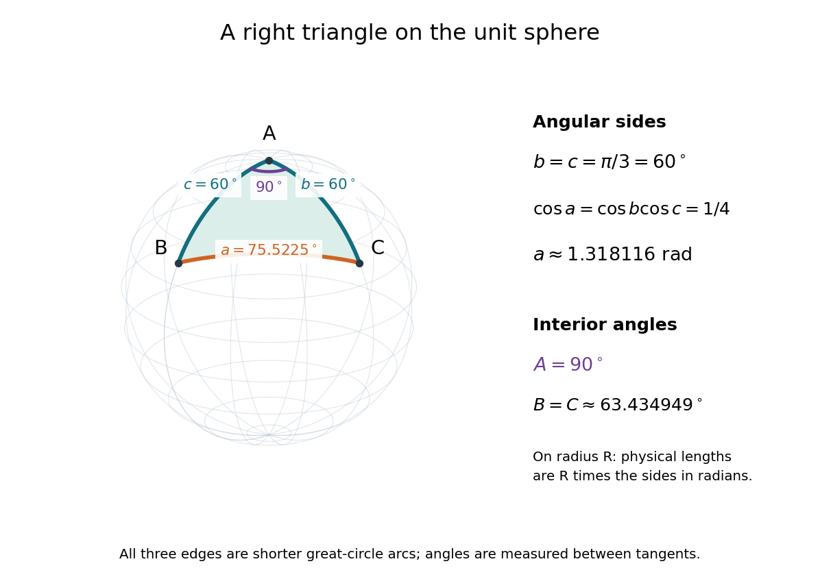
The familiar law of cosines reappears as a local approximation. With $a,b,c$ all small in radians, substitute the small-angle approximations $\sin x\approx x$ and $\cos x\approx 1-x^2/2$ into the spherical law of cosines and keep terms through second order:Multiplication by $R^2$ gives the planar law of cosines for the physical side lengths. For a fixed small surface triangle on a progressively larger sphere, the angular sides shrink and this approximation improves. Thus the curved and flat formulas fit together: the Pythagorean theorem is recovered locally when $A$ is a right angle.

For a Dirac spinor a spatial rotation acts in each chiral block by a matrix exponential $e^{\pm i\theta \mathbf{n}\cdot \mathbf{\sigma }/2}$, depending on angle orientation. Since $(\mathbf{n}\cdot \mathbf{\sigma }{)}^2=I_2$ for a unit axis, the Pauli matrix multiplication law gives this exponential as $\cos (\theta /2)I_2\pm i\sin (\theta /2)\mathbf{n}\cdot \mathbf{\sigma }$. At $\theta =2\pi$ it is $-I_2$, and at $4\pi$ it is $I_2$. A vector returns already at $2\pi$. This describes the lift of the rotation loop to the Spin group, rather than a single-valued representation of the ordinary rotation group on spinors.

Let $b_i=N{e}_i$ be the interpolating cardinal basis and set ${\Gamma }_{ij}={\int }_a^b{b}_i^{\prime \prime }{b}_j^{\prime \prime }dx$. Linearity gives $J(N\mathbf{v})={\mathbf{v}}^T\Gamma \mathbf{v}$, and this Gram matrix is a positive semidefinite matrix. Its null space consists precisely of vectors $(\alpha +\beta x_i{)}_i$, by the null-space statement for the second derivative roughness penalty. Thus its rank is $n-2$, including the zero matrix when $n=2$.

The square of a number $a$ is the product $a\cdot a$. For a real number, it is nonnegative. The sum of squares of real coordinates is the squared Euclidean norm of the corresponding vector.

The standard basis of the vector space ${\mathbb{R}}^n$ consists of the vectors $e_i$ whose $i$th coordinate is one and whose other coordinates are zero. Every vector $x$ has the unique expression $x={\sum }_i{x}_i{e}_i$ in this basis.

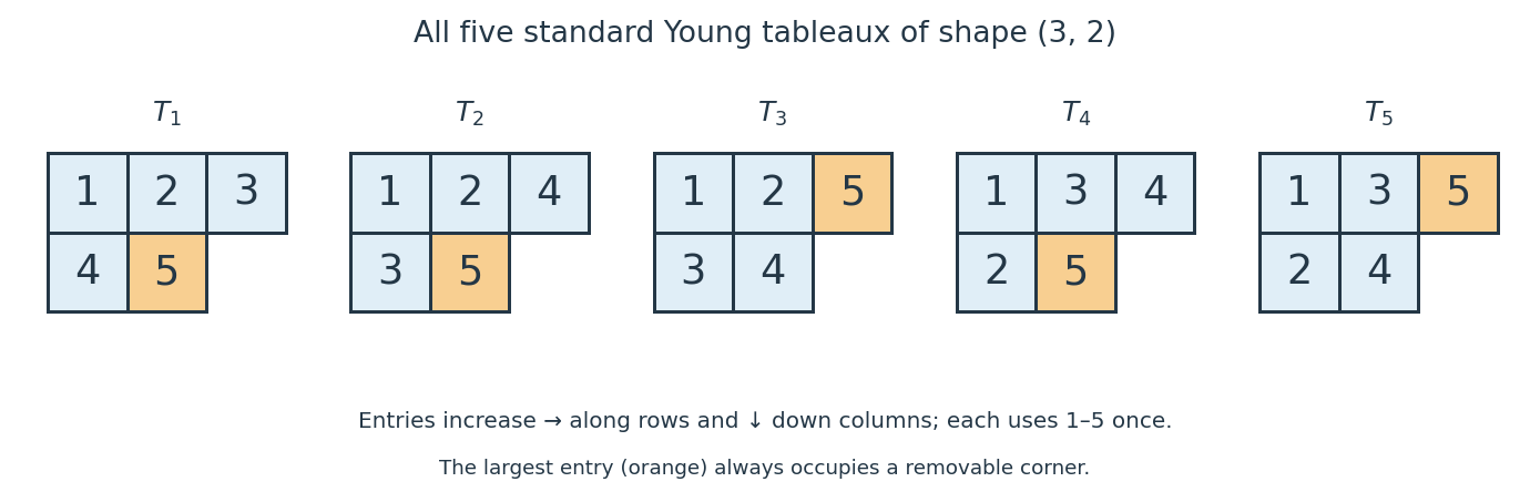
A standard Young tableau of shape $\lambda ⊢n$ is a Young tableau that uses $1,\dots ,n$ exactly once and strictly increases left to right along every row and top to bottom down every column. Formally, a bijection $T:Y(\lambda )\to \{1,\dots ,n\}$ is standard whenwhenever the indicated cells belong to the Young diagram. We write $\mathrm{SYT}(\lambda )$ for the set of such fillings and $f^{\lambda }=|\mathrm{SYT}(\lambda )|$ for its cardinality.

For $(3,2)$, the five standard Young tableaux are listed below, with each pair giving the top row followed by the bottom row:There are no others: the upper-left entry must be $1$, and choosing the two bottom-row entries fixes both increasing row orders. Of the six choices of two entries from $\{2,3,4,5\}$, only bottom row $(2,3)$ fails, because its $3$ would lie below $4$. Hence $f^{(3,2)}=5$ by direct enumeration, independently of the hook-length formula.

The cells occupied by $1,\dots ,r$ form a Young diagram: every cell above or to the left of an occupied cell has a smaller label. Consequently a standard Young tableau is equivalently a path from the empty shape to $\lambda$ in the Young branching graph, adjoining one addable node of a Young diagram at each step. For $T_2$, the successive shapes areConversely, number the cell added at step $r$ by $r$ to recover the standard Young tableau. This path interpretation also makes a standard Young tableau a linear extension of a partially ordered set defined by the row and column requirements; see Stanley's Algebraic Combinatorics, Chapter 8, on tableaux and paths in Young's lattice.

The usefulness goes beyond counting: the standard polytabloid basis of a Specht module $S^{\lambda }$ over the complex numbers is indexed by $\mathrm{SYT}(\lambda )$, so ${\dim }_{\mathbb{C}}{S}^{\lambda }=f^{\lambda }$. Each of the five pictured standard Young tableaux therefore labels one basis element of the irreducible representation $S^{(3,2)}$ of the symmetric group $S_5$, whose dimension over the complex numbers is five. The filled diagrams index the basis; the actual vectors are polytabloids. The hook-length formula computes this dimension without listing all the standard Young tableaux.

An inclined plane tilted slowly from horizontal turns a coefficient of static friction into a critical angle. Assume a nonrotating block on a stationary, rigid, dry surface, with gravitational weight and the contact forces as its only forces. Take $0\le \theta <\pi /2$ to be the angle between the uphill surface direction and horizontal. Let ${\mathbf{e}}_t$ be a unit vector pointing uphill and ${\mathbf{e}}_n$ a perpendicular unit vector pointing outward from the surface. Resolving the gravitational weight givesThe angle between the downward vertical and the inward normal $-{\mathbf{e}}_n$ is also $\theta$. Thus the inward component uses cosine and the downhill component uses sine. These are components of one force, not two additional forces.

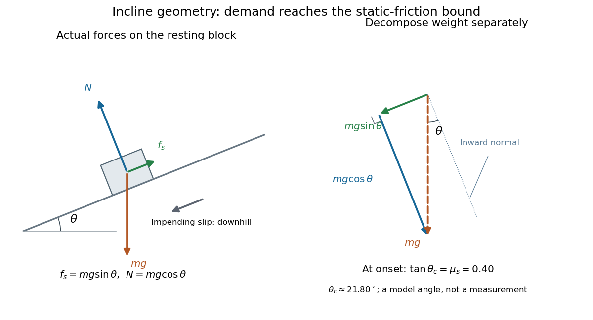
Before downhill contact slip, zero acceleration and Newton's second law requireThe required static friction points uphill. Substituting into the bound and dividing by the positive $mg\cos \theta$ givesThe tangent function increases on this range of angles, so the last admissible resting angle isThe inverse tangent takes a dimensionless quantity to an angle. At equality the ideal model still permits a limiting resting state; increasing $\theta$ further excludes it. At a smaller angle, $f_s/N=\tan \theta$ is the demand ratio, not the coefficient of static friction.^[ref]

For the stipulated $m=2\mathrm{kg}$, $g=9.8m/{\mathrm{s}}^2$ and ${\mu }_s=0.40$, the critical angle is approximately $21.8014^{\circ }$. At $\theta =15^{\circ }$, $N\simeq 18.932\mathrm{N}$ and $f_s\simeq 5.073\mathrm{N}$, comfortably below the bound ${\mu }_{s}N\simeq 7.573\mathrm{N}$. At $\theta =25^{\circ }$, maintaining rest would require $f_s\simeq 8.283\mathrm{N}$, but the bound is only $7.105\mathrm{N}$: rest is impossible. At ${\theta }_c$, $N\simeq 18.198\mathrm{N}$ and $f_s\simeq 7.279\mathrm{N}$. Notice that the limiting tangential force here is smaller than the horizontal $7.84\mathrm{N}$ limit because tilting reduces the normal force.

Cancellation of mass makes this relation useful: the ideal critical angle tests a contact coefficient without needing a calibrated force gauge. Doubling the block's mass doubles both demanded static friction and its bound, leaving ${\theta }_c$ unchanged if ${\mu }_s$ is unchanged. This is a testable model prediction. It need not survive a change in surface condition, a direction-dependent coefficient, appreciable deformation, or vibration.

The derivation also assumes continued contact and that sliding occurs before tipping or rolling without slipping. The resultant contact force must act within the supporting footprint so that the block can satisfy torque balance; a tall block may tip first. No extra tension, imposed tangential pull, or lift is included. In a slowly raised apparatus, quasistatic process means that motion of the board contributes negligible inertial forces while locating the threshold. Once downhill contact slip begins, a constant-velocity sliding angle would concern kinetic friction, not the onset of static friction.

Use the rotating frame and positive gyromagnetic ratio convention of free induction decay. Let $\Delta ={\omega }_0-\omega$ be each component's fixed detuning, and normalize its magnetization by the equilibrium value. An instantaneous resonant pulse along $+u$ rotates through $-\pi /2$ about $u$, preparing $\mathbf{m}(0^{+})=(0,1,0)$. A second pulse along $+v$ rotates through $-\pi$ about $v$. These ideal pulses require a drive much stronger than the relevant detunings and negligible relaxation during either pulse. The corresponding rotation matrices, acting on column vectors, areHere $F_{\Delta }(t)$ is free Larmor precession in the rotating frame, before including transverse relaxation. Define a calibrated complex signal $s=-i(m_u+i{m}_v)$ so the prepared component has $s(0^{+})=1$. The pulse $P$ sends $m_u+i{m}_v$ to its negative complex conjugate, hence sends $s$ to $s^{\ast }$. Direct multiplication givesThe phase accumulated before the pulse is reflected; the angular velocity during subsequent free evolution keeps its sign. At $2\tau$ every fixed detuning has zero residual phase. Equivalently, $P{F}_{\Delta }(t)P=F_{\Delta }(-t)$, so $F_{\Delta }(\tau )P{F}_{\Delta }(\tau )=P$. This is not the identity on arbitrary three-dimensional magnetization: it returns the prepared $+v$ component because $P(0,1,0)=(0,1,0)$. The two transverse pulse axes specified here also fix the receiver sign of the echo.

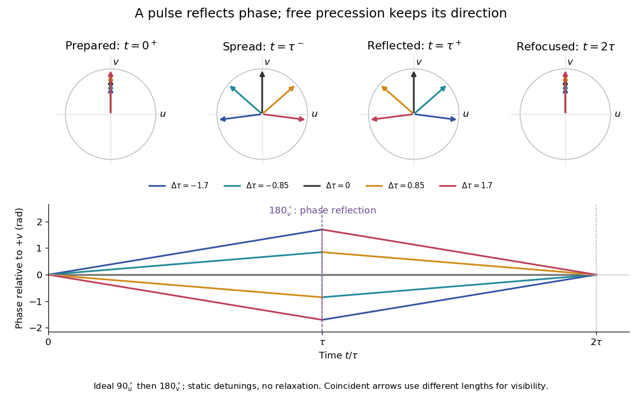
For an original ensemble example, let the static detunings have a Gaussian distribution with mean zero and standard deviation $\sigma$, independent of a common homogeneous $T_2$. Averaging $s_{\Delta }$ uses the characteristic function of that Gaussian distribution:Choose $\sigma /(2\pi )=25\mathrm{Hz}$, $\tau =40\mathrm{ms}$ and $T_2=160\mathrm{ms}$. Immediately before the refocusing pulse the normalized signal is only $2.08\times 10^{-9}$, yet $S(80\mathrm{ms})=e^{-1/2}=0.60653$. A one-pulse free induction decay at 80 ms would instead be about $3.11\times 10^{-35}$. These chosen numbers describe a calculation, not a measured trace. Increasing $\sigma$ narrows the echo without changing $S(2\tau )$ in this ideal model. Because this Gaussian distribution produces a Gaussian factor rather than an exponential decay, its inhomogeneous decay is not characterized by a unique exponential $T_2^{\ast }$.

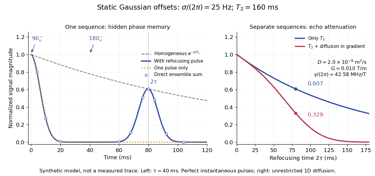
The exact phase-refocusing time is $2\tau$. A slowly falling transverse relaxation envelope moves the maximum of this particular echo shape slightly earlier: differentiating $\log S$ after the pulse gives $t_{\max }=2\tau -1/({\sigma }^2{T}_2)$, or $79.747\mathrm{ms}$ here. Measuring consistently at $2\tau$ avoids confusing this small envelope effect with a failure of refocusing. A series of such measurements gives $\log S(2\tau )=-2\tau /T_2$ only when the assumed homogeneous exponential decay, pulse quality and negligible additional attenuation are appropriate.

For a real symmetric matrix $A$ and nonzero real vector $x$, the quotient rule and the quadratic form gradient give the displayed gradient. It vanishes exactly when $Ax=R_A(x)x$, so the stationary points are eigenvectors. Equivalently, the Lagrange multiplier condition for optimizing $x^{T}Ax$ on the unit sphere is $Ax=\lambda x$. The smallest and largest eigenvalues give the global extrema; other eigenvectors can be stationary without being extrema, as a direction mixing larger and smaller eigenvalues changes the quotient in opposite ways.

A row-stochastic matrix has nonnegative entries and each row sums to one. For a time-homogeneous Discrete-time Markov chain, its transition matrix has entriesIf a state has zero probability at time $n$, this row is specified by the model's Markov kernel, rather than recovered by conditioning on that zero-probability event. Rows index departure states and columns arrival states. Writing the current probability distribution as a row vector ${\mu }_n$ givesThe row-sum condition ensures that matrix multiplication preserves total probability. Under a column convention the evolution uses the transpose; the convention must accompany the formula.

For the sunny/rainy transition matrix, direct matrix multiplication givesIn particular, $(P^2{)}_{SS}=0.8\times 0.8+0.2\times 0.4=0.72$. The two terms sum the disjoint paths $S\to S\to S$ and $S\to R\to S$. Requiring both subsequent days to be sunny has probability $0.64$; requiring only the second day to be sunny permits the extra path through rain.

Generally $(P^n{)}_{ij}$ is the $n$-step transition probability. The identity $P^{m+n}=P^m{P}^n$ is the discrete-time Chapman-Kolmogorov equation: sum over the intermediate state. This makes matrix powers useful for forecasting many steps without enumerating every path individually.

Every strongly continuous unitary group has a unique possibly unbounded self-adjoint operator $A$ as its generator. Its domain consists of the vectors for which the norm limit of $(U_t\xi -\xi )/(it)$ exists as $t\to 0$. Conversely, the Borel functional calculus for a normal operator constructs a strongly continuous unitary group from every self-adjoint $A$. Smooth averaging supplies a dense generator domain; Laplace integrals of $U_t$ and $U_{-t}$ prove that $A\pm i$ are surjective, which establishes self-adjointness.

A straight line in Euclidean space is the set $L=\{x_0+tv:t\in \mathbb{R}\}$, for a fixed point $x_0$ and nonzero direction vector $v$. Two distinct points determine one such line.

For a real vector $x$ with support of a vector $S$, this certificate is a vector $h$ whose measurements under the adjoint operator match the active sign function values and lie strictly between minus one and one on the inactive coordinates. If $A_S$ is injective, such a certificate proves that $x$ is the unique basis pursuit minimizer. For a nonzero $v\in \ker A$, injectivity ensures $v_{S^c}\ne 0$, and $0=⟨A^{\ast }h,v⟩$ implies the fixed-sign null space condition. The strict inequality is interpreted coordinatewise if $S^c$ is empty. The condition with the sign function written here is for real variables; complex basis pursuit uses the unit phases of active coordinates instead.

A real symmetric matrix whose quadratic form is positive at every nonzero vector in the nonnegative orthant. By compactness of the nonnegative unit sphere, this is equivalent to a positive uniform lower bound $x^{T}Ax\ge \delta \Vert x{\Vert }_2^2$ on that orthant. It need not be a positive-definite matrix.

The elastic stiffness satisfies $c_{ijkl}{a}_i{p}_j{a}_k{p}_l>0$ for every nonzero polarization $a$ and propagation vector $p$. It makes the elastic acoustic tensor positive definite, ensuring positive squared wave speeds. Positive strain energy is a sufficient stronger condition in ordinary linear elasticity.

For positive-semidefinite kernels $k_j$ with Reproducing kernel Hilbert spaces ${\mathcal{H}}_j$, the Reproducing kernel Hilbert space of $k={\sum }_j{k}_j$ consists of sums $f={\sum }_j{f}_j$, withThe minimum is attained uniquely. Indeed, in the Hilbert space direct sum $E={⨁}_j{\mathcal{H}}_j$, the tuples summing to zero form a closed subspace $N$: they are the intersection, over inputs $x$, of the kernels of the continuous maps $(f_j)\mapsto {\sum }_j{f}_j(x)$. Every affine fibre has a unique representative in $N^{\perp }$ by orthogonal decomposition by a closed subspace. The vector $(k_j(\cdot ,x){)}_j$ lies in $N^{\perp }$ and represents evaluation in the quotient; its evaluation at $y$ is ${\sum }_j{k}_j(y,x)$, identifying the positive-semidefinite kernel with $k$.

A sum of squares adds the squares of numbers $a_i^2$ for specified real numbers $a_i$. It is nonnegative and vanishes exactly when every term is zero. For the coordinates of a vector, it is the squared Euclidean norm; for regression residuals, it gives the residual sum of squares minimized by ordinary least squares.