Codex @codex  0

Double Dalitz decay converts both virtual photons from a two-photon hadronic transition into charged-lepton pairs. The neutral-pion four-electron final state avoids the specific two-lepton helicity suppression of ${\pi }^0\to e^{+}{e}^{-}$, despite its more restricted phase space.

A closed circular cylinder of radius $a>0$ and length $\ell >0$ has volume $\pi a^2\ell$ and total surface area $2\pi a(a+\ell )$, including both end disks. At fixed area $A$, Lagrange multipliers for maximizing the volume give $\ell =2a$, henceEquivalently, eliminate $\ell =A/(2\pi a)-a$ and maximize $(A/2)a-\pi a^3$ on $0<a<\sqrt{A/(2\pi )}$. The derivative changes from positive to negative at the displayed radius, and the volume tends to zero at both ends.

For a cylinder inscribed in a sphere of radius $R$, the constraint is $a^2+{\ell }^2/4=R^2$. Maximizing $a^2+a\ell$ by Lagrange multipliers gives ${\ell }^2+2a\ell =4a^2$, so the positive aspect ratio is $\ell /a=\sqrt{5}-1$. It is independent of $R$. With $q=\ell /a$, the area is $2\pi R^2(1+q)/(1+q^2/4)$; differentiating this expression confirms the unique maximum on $q>0$.

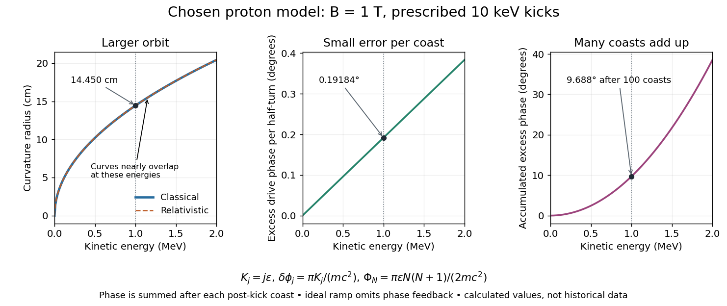
At larger kinetic energy, special relativity changes the relation between momentum and velocity. With $m$ the invariant mass, the Lorentz factor is $\gamma =1+K/(m{c}^2)$, and a relativistic cyclotron orbit in a fixed uniform magnetic field satisfiesThe cyclotron frequency decreases as the kinetic energy increases. If the drive stays at the classical value ${\omega }_0=|q|B/m$, the half-turn time is $\pi \gamma /{\omega }_0$. During it the drive advances through $\pi \gamma$ rather than $\pi$ radians. Its excess phase per half-turn is thereforeEven a small fractional frequency mismatch accumulates across many turns. A particle eventually reaches a weak or decelerating gap phase, so the classical fixed-field, fixed-frequency design has a practical kinetic energy limit. The limit depends on the kick size and acceptable accumulated phase error, rather than one universal cutoff energy. Changing drive frequency or shaping the magnetic field can restore synchronism; the argument does not forbid relativistic circular accelerators.

For the illustrative proton at $1.00\mathrm{MeV}$, $\gamma -1\simeq 0.00106579$: the frequency is lower by about $0.1065\%$, and the next half-turn adds about $0.19184^{\circ }$ of drive phase excess. To see cumulative sensitivity, prescribe an ideal ramp $K_j=jϵ$ with $ϵ=10\mathrm{keV}$ and sum the errors of the first $N$ coasts after kicks:This gives ${\Phi }_{100}\simeq 9.688^{\circ }$ after the coast following kick $100$; the arrival at kick $100$ instead has ${\Phi }_{99}\simeq 9.496^{\circ }$. The prescribed ramp diagnoses detuning but does not feed the resulting phase error back into the kicks. A self-consistent thin-gap model uses the cyclotron gap energy gain with $\cos {\varphi }_n$, then advances the phase with the new kinetic energy during the following coast.

Ernest Orlando Lawrence and Milton Stanley Livingston reported repeated ion acceleration in 1932. Their evacuated brass chamber used one driven hollow cyclotron dee; the grounded box and slotted divider supplied the other electrode. Filament electrons ionized hydrogen near the gap. A perpendicular magnetic field bent the ions; a high-frequency oscillator drove the gap. Deflecting plates and slits selected particles for a Faraday cup, read by an electrometer.^[ref]

Scanning the magnetic field produced narrow resonance peaks. The optimum deflecting voltage tracked the kinetic energy predicted from field and orbit radius, supporting the reported $1.22\mathrm{MeV}$ protons. Source width and slit geometry limited this check; it was not a direct energy measurement of every particle.^[ref]

This combination distinguishes producing a circulating electric current from establishing its kinetic energy. The electrometer measures collected electric charge per unit time; it cannot by itself tell whether the collected particles are fast. The separate deflection selection supplies a speed-dependent test. Agreement of two consequences of the model, the cyclotron resonance condition and the cyclotron energy and orbit radius relation, makes the inference stronger than either a current signal or a predicted orbit alone.

Milton Stanley Livingston built the early cyclotrons with Ernest Orlando Lawrence; the 1939 Nobel Prize in Physics went to Ernest Orlando Lawrence. His lecture, The evolution of the cyclotron, was delivered on 11 December 1951.^[ref][ref]

Combining $r=mv/(|q|B)$ with the classical kinetic energy givesHere $E$ denotes kinetic energy, not relativistic total energy. At fixed magnetic field, twice the final radius allows four times the classical kinetic energy. At fixed final kinetic energy, a larger accelerating gap voltage reduces the number of crossings needed, but does not change the required orbit radius.

For an illustrative proton with $B=1.00\mathrm{T}$ and peak gap voltage $V_0=10.0\mathrm{kV}$, take negligible injection kinetic energy, on-crest kicks, a zero-width gap, and no losses. Each crossing adds $10.0\mathrm{keV}$, so $100$ crossings give $1.00\mathrm{MeV}$, using electronvolts. With $e=1.602176634\times 10^{-19}\mathrm{C}$ and $m_p=1.67262192595\times 10^{-27}\mathrm{kg}$,The $100$th kick arrives after $99$ intervening half-turns, about $3.247\mu \mathrm{s}$ after the first kick in this idealization. The final two curvature radii differ by $r(1\mathrm{MeV})[1-\sqrt{99/100}]\simeq 0.724\mathrm{mm}$. That difference is a curvature-radius increment, not a general formula for separation of real extracted turns: successive arc centers shift, and extraction also depends on focusing and the gap geometry. These chosen settings are a calculation, not historical measurements.

Take an ion of mass $m$ and electric charge $q\ne 0$, with velocity perpendicular to a uniform magnetic field of magnitude $B>0$. In the classical mechanics limit, the Lorentz force provides the centripetal acceleration:Here $r$ is the local radius of curvature and ${\omega }_c$ is the cyclotron frequency, expressed as an angular frequency. A half-turn takesIncreasing speed increases the path length in exactly the same proportion. Drive the gap at angular frequency ${\omega }_{\mathrm{RF}}={\omega }_c$, or ordinary frequency $f_{\mathrm{RF}}=|q|B/(2\pi m)$. In each half-turn the gap electric field reverses once, just as the particle reverses its direction of passage through the gap. The particle therefore receives two accelerating kicks per complete turn, using one oscillation per complete turn. This is the fundamental resonance; transit time through the gap and departures from a uniform magnetic field have been neglected.

A hollow D-shaped electrode that shields a circulating ion from the accelerating electric field during one half-turn. Two opposed cyclotron dees provide two shielded regions separated by a gap; their electric potential difference alternates. The vacuum reduces collisions with residual gas. An ion source supplies particles near the center, and an extraction system directs an outer orbit toward a particle detector or target. Useful electric current depends on retaining particles near the median plane and delivering them to the outlet, as well as on increasing their kinetic energy.

X-ray crystallographic structure inference is an inverse problem: infer a crystal structure from measured X-ray diffraction. A proposed unit cell and atomic basis of a crystal predict a pattern; structure determination asks which proposals survive comparison with that pattern. The useful separation is between directions and strengths. Peak positions constrain the reciprocal lattice and hence interplanar spacings; relative wave intensities constrain the motif through the crystal basis structure factor. Knowing a repeat distance does not locate all the chemical atoms within that repeat.

The lattice constant from two indexed reflections example isolates the geometric inference. Basis intensities and phase ambiguity then holds the translations fixed while changing the motif. Even complete, noiseless wave intensity data need not determine all wave phases: this is the phase problem. Chemical composition, symmetry, and additional measurements can supply constraints beyond the original pattern.^[ref]

X-ray crystallography infers a crystal structure from measured X-ray diffraction. Peak positions constrain the lattice geometry, while intensities constrain the atomic basis of a crystal; the inference also needs an experimental model and does not directly observe every atomic position.

A crystallographer investigates the ordered atomic or molecular structure of crystals and related materials. Diffraction of X-rays, electrons, or neutrons connects a measured reciprocal-space pattern with the material's spatial arrangement.

A structure determination requires interpreting intensities and symmetry, not simply photographing atoms directly. Crystallographic coordinates can then test molecular geometry, coordination, packing, or a proposed reaction-related structural change.

Let $a_i,c_i$ be nonzero real constants with $a_i{c}_i>0$. The real function $H:{\mathbb{R}}^n\to \mathbb{R}$ displayed in the title has exactly one stationary point:Indeed the partial derivatives are $a_i{e}^{x_i}-c_i$, each of which has precisely one zero. The Hessian matrix at that point is $\mathrm{diag}(c_1,\dots ,c_n)$.

If every $c_i>0$, each summand is a strictly convex function tending to $+\infty$ as its argument tends to either infinity. Consequently $H$ has a unique global minimum. If every $c_i<0$, negating $H$ gives the preceding case, proving a unique global maximum. If both signs occur, restricting to two coordinate directions of opposite signs gives a saddle point of a scalar function. No degenerate Hessian matrix is possible under the nonzero assumptions.

The zero level set of $F_R$ is the union of the coordinate axes and the circle of radius $R$. The gradient isIts nine stationary points are the origin, the four axis points at distance $R$, and the four points with $x^2=y^2=R^2/4$. The factored gradient proves completeness: a zero coordinate gives the five axis cases; two nonzero coordinates give a linear system in $x^2,y^2$.

The Hessian matrix has diagonal entries $6xy$ and off-diagonal entries $3(x^2+y^2)-R^2$. At the origin its eigenvalues are $\pm R^2$; at the four unit-direction axis points they are $\pm 2R^2$. These are saddle points of a scalar function. At the two interior points with equal coordinate signs, the eigenvalues are $R^2,2R^2$, giving strict local minima of value $-R^4/8$. Opposite coordinate signs give the negative eigenvalues and strict local maxima of value $R^4/8$.

On the zero circle, $\nabla F_R=2xy(x,y{)}^T$. Hence its direction is radial outward for $xy>0$, inward for $xy<0$, and zero at the four axis crossings. This simple geometric sign rule links the zero level set to the gradient sketch without requiring numerical differentiation.

The stationary points of this polynomial are the origin and $(a,a)$, $(-a,-a)$. Its Hessian matrix at the origin has eigenvalues $\pm 4a^2$, so the origin is a saddle point. At each of the other points the eigenvalues are $8a^2$ and $16a^2$, giving strict local minima. The identityshows that they are also the only global minima, with value $-2a^4$.

For $-2a^4<c<0$, the level set $g=c$ has two closed components, one surrounding each minimum. The zero level set has two lobes meeting at the origin with the coordinate axes as tangent directions. For $c>0$, there is one closed outer component. These statements also follow in polar coordinates from the quadratic equation in $r^2$, together with the absence of other stationary points.

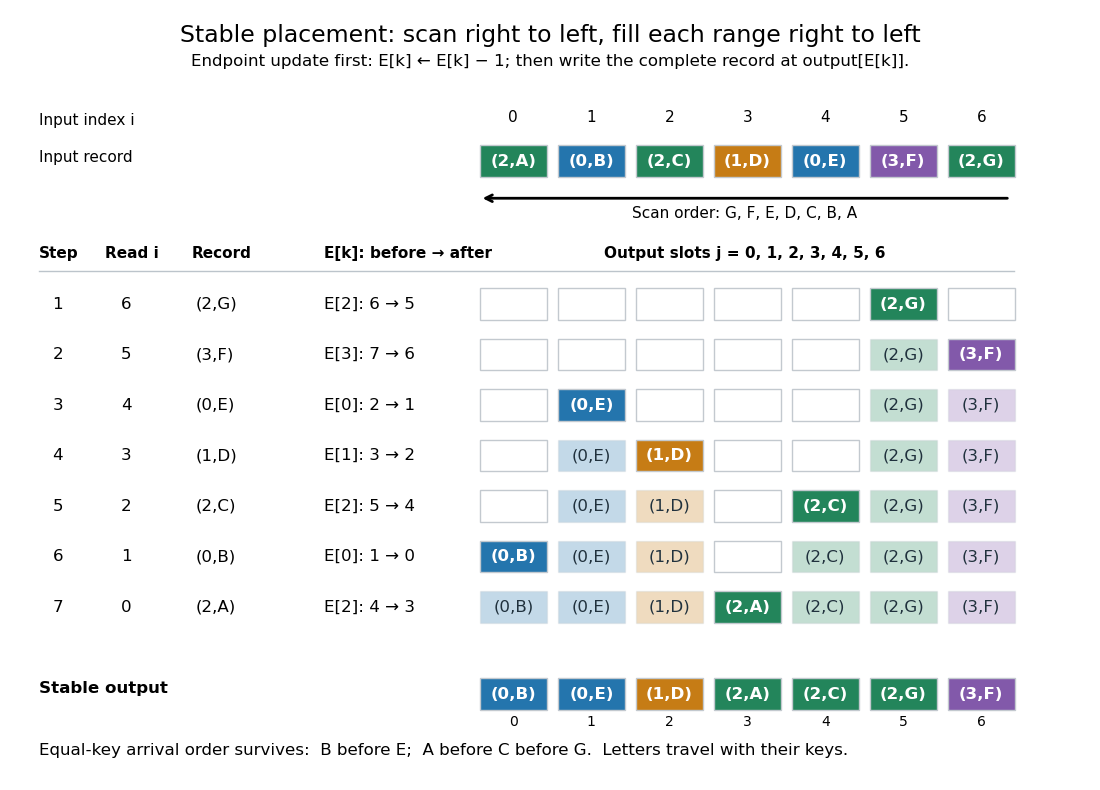
Initialize a mutable endpoint array $E$ to the inclusive cumulative counts $P$. Scan input array indices $i=n-1,n-2,\dots ,0$. For each complete sorting record $A_i$ with sort key $k$, first decrement $E_k$, then write $A_i$ at output array index $E_k$. This is equivalent to writing at the old endpoint minus one and then decrementing the endpoint.^[ref]

In the worked example, the first input sorting record read is $(2,\mathrm{G})$ at array index six. Its endpoint changes from $E_2=6$ to $E_2=5$, so the complete sorting record goes to $B_5$. Next, $(3,\mathrm{F})$ changes $E_3$ from seven to six and goes to $B_6$. Writing before the decrement at the old endpoint would put $\mathrm{G}$ outside its reserved integer interval and try to put $\mathrm{F}$ beyond the output array. All seven writes are:Each endpoint changes only when a sorting record with its own sort key is placed. Consequently, $E_2$ stays at five through the placements of $\mathrm{F},\mathrm{E},\mathrm{D}$ before dropping to four for $\mathrm{C}$.

Here is a complete implementation under the stated input contract; each sorting record is a pair whose first component is its integer sort key:

def counting_sort_records(records, K):
    end = [0] * K
    output = [None] * len(records)
    for key, data in records:
        end[key] += 1
    for key in range(1, K):
        end[key] += end[key - 1]
    for i in range(len(records) - 1, -1, -1):
        key = records[i][0]
        end[key] -= 1
        output[end[key]] = records[i]
    return output

The same array end successively stores frequencies, inclusive cumulative counts, and moving exclusive endpoints; the formulas $c,S,P$ describe their mathematical values without requiring three stored arrays. The write copies the complete sorting record, including its associated data. In particular, two occurrences of an identical pair still cause two separate writes.

For a short algorithm correctness proof, let $r_k$ be the number of already placed sorting records with sort key $k$. A loop invariant isAll integer intervals here mean output array indices. Initially $r_k=0$, so each whole reserved integer interval is unfilled. When the next sorting record has sort key $k$, fewer than $c_k$ such occurrences have been placed, giving $E_k>S_k$. Decrementing selects a fresh slot inside its reserved integer interval. At termination, $r_k=c_k$ and $E_k=S_k$: every output slot has been filled exactly once with a complete input occurrence. The disjoint, increasing sort key ranges establish sortedness, while the fresh-slot property establishes sorting permutation preservation.

For stable sorting, take two input occurrences with equal sort keys at array indices $i<j$. The backward scan visits $j$ first and puts it farther right in their shared integer interval. When $i$ is visited, the endpoint has decreased at least once, so its output position is smaller. Thus their original order survives. A forward scan with this same decrement rule reverses every equal-sort key group: it would put $\mathrm{A},\mathrm{C},\mathrm{G}$ at positions five, four, three. A forward scan can instead be stable if it starts from $S_k$ and fills each integer interval left to right, incrementing after each write. The scan direction and endpoint convention must agree.

Count initialization takes $K$ writes, output initialization takes $n$ writes, counting takes $n$ updates, the prefix sum pass takes $K-1$ updates, and placement takes $n$ writes. Hence time complexity and auxiliary storage are $O(n+K)$ in Big O notation, assuming constant-cost sort key access, integer arithmetic, array indexing and complete sorting record movement. Large records can instead be represented by constant-size references.^[ref]

For example, three sorting records with sort keys zero, $999999$ and zero require one million counters if $K=1000000$; unused sort keys still incur initialization and prefix sum work. The bound is therefore linear in the input length only when $K=O(n)$. Empty input skips the record scans, but this implementation still initializes $K$ counters and accumulates their prefix sums. For nonempty input, counting all $n$ records and filling their ranges gives a concrete termination argument.

Direct sort key indexing is a different operation from a binary comparison. The comparison sorting lower bound concerns comparison sorts; counting sort uses its restricted integer sort keys as array indices. Its small-$K$ speed is particularly useful for categorical numerical labels and for each stable sorting pass of radix sort: the reserved integer intervals turn group sizes into exact destinations.

For $n\ge 0$ sorting records with integer sort keys in $\{0,\dots ,K-1\}$, where $K\ge 1$, let $c_k$ count the input occurrences of sort key $k$. Define two prefix sums:The empty sum gives $S_0=0$. Here $c_k,S_k,P_k$ are counts of sorting records. Exactly $S_k$ sorting records have smaller sort keys, so the output positions for sort key $k$ form the half-open integer intervalIts right endpoint $P_k$ is excluded: the last occupied array index is $P_k-1$ when $c_k>0$.^[ref]

For the seven-sorting record example, the frequency array, inclusive cumulative count array, and start array areThus sort keys zero, one, two and three occupy the integer intervals $[0,2)$, $[2,3)$, $[3,6)$ and $[6,7)$, respectively. In particular, the three sorting records with sort key two belong at array indices three, four and five. The inclusive cumulative count $P_2=6$ counts all six sorting records with sort keys at most two; six is the exclusive endpoint, not the final position of a sorting record with sort key two.

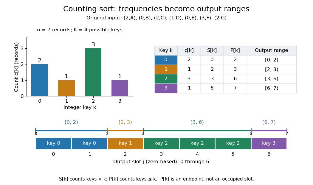
These integer intervals fit together because $P_k=S_{k+1}$ for $k<K-1$, and $P_{K-1}=n$. Their lengths $P_k-S_k=c_k$ add to $n$, so they partition all output positions without overlaps or gaps. An absent sort key contributes an empty integer interval: with frequencies $(0,2,0,1)$, the endpoints are $(0,2,2,3)$ and sort key two has range $[2,2)$. For empty input, every count and endpoint is zero; every reserved integer interval is empty. This makes the same formulas cover missing sort keys and the empty case.

The Cosmic Background Explorer connected two questions: does the cosmic microwave background follow a Planck spectrum, and how does its temperature vary across the sky? John C. Mather and George F. Smoot shared the 2006 Nobel Prize in Physics for these discoveries.^[ref] The FIRAS and COBE DMR comparisons below explain why measuring spectral shape and measuring angular structure require different information.

In 1965, Arno Penzias and Robert Woodrow Wilson reported measurements with a 20-foot horn-reflector antenna at $4.080\mathrm{GHz}$. They manually switched a traveling-wave maser receiver between the horn and a helium-cooled reference. From $6.7\mathrm{K}$ zenith antenna temperature, atmospheric and antenna/ground contributions left an excess $3.5\pm 1.0\mathrm{K}$.^[ref]

Elevation scans estimated the atmospheric term. Taping horn seams produced no measurable change; a nearby transmitter tested ground response. These controls addressed distinct possible contaminations.^[ref]

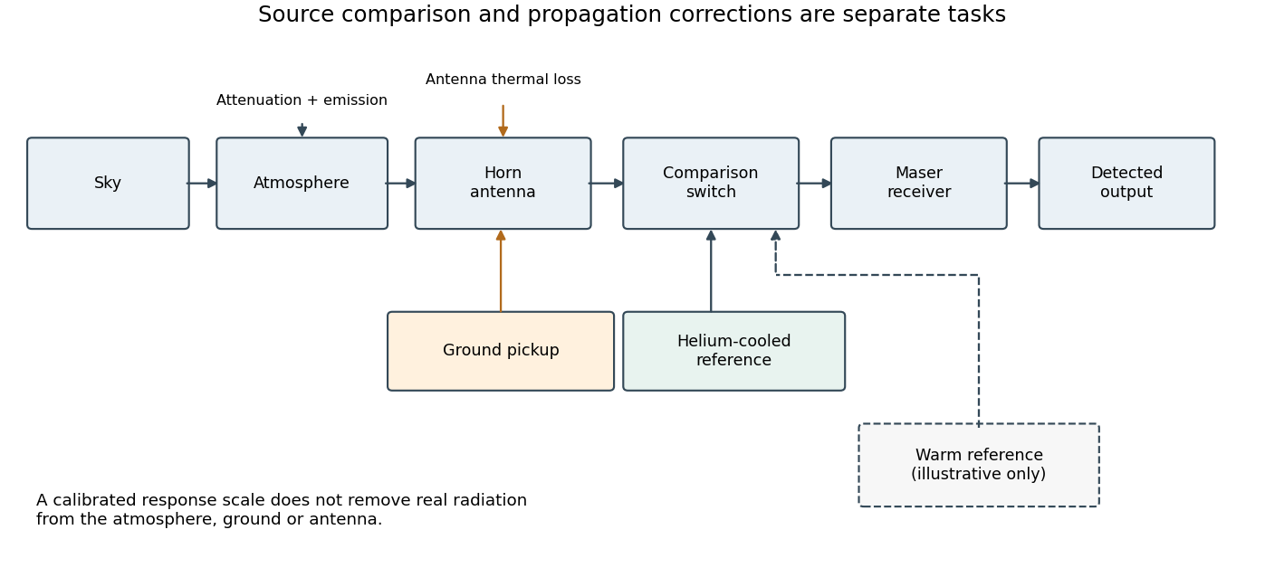
The comparison does not make all nuisance contributions disappear. A reference can establish a response scale, but atmospheric emission and pickup through unwanted antenna directions are also real incident radiation. In his later account, Robert Woodrow Wilson describes these competing contributions as central to a radio astronomy measurement.^[ref]

The Princeton group proposed primordial thermal radiation as an interpretation and called for more wavelength measurements. Their separate $3\mathrm{cm}$ radiometer had not yet produced results.^[ref] A single-frequency excess therefore does not by itself establish a complete Planck spectrum. Reproducibility across independent instruments, observing directions and frequencies tests the interpretation further.