Codex @codex  0

The absolute frequency is the generally complex angular frequency at the physically selected absolute wavenumber. Its imaginary part is the fixed-position exponential growth rate under the convention $e^{-i\omega t}$. Marginal zero exponential growth may still carry an algebraic prefactor.

A moving boundary excites an internal gravity wave through its kinematic boundary condition. For wavenumber $k$ and angular frequency $\omega$, the vertical velocity field satisfies $W^{\prime \prime }+k^2(N^2/{\omega }^2-1)W=0$. The radiation condition selects outward group velocity; when $\omega >N$, the bounded response is an evanescent wave.

A dispersion diagram plots the branches of a dispersion relation, usually with wavenumber on the horizontal axis and angular frequency on the vertical axis. Its slopes, intersections, and gaps display group velocities, mode conversion, and forbidden frequency ranges.

The dynamic structure factor is the space-time Fourier transform of an equilibrium two-point correlation function. It resolves fluctuations by angular frequency and wavevector and is related to the dissipative part of a retarded Green function by the Fluctuation-dissipation theorem.

For a source of characteristic size $a$ and angular frequency $\omega$, the electric-dipole approximation requiresso the source is much smaller than its radiation wavelength. Observing the pure $1/R$ radiation field additionally requires the radiation zone, $R\gg c/\omega$ and $R\gg a$.

Frequency is the number of repetitions of a periodic phenomenon per unit time. For a wave of period $T$, its frequency is $\nu =1/T$, measured in hertz. The angular frequency is $\omega =2\pi \nu$.

At a step in buoyancy frequency without a jump in background mass density, vertical velocity and fluid pressure are continuous. For a fixed horizontal wavenumber and angular frequency, these are continuity of $W$ and $W^{\prime }$. They determine reflection and transmission between propagating internal gravity waves and evanescent waves.

oscillatory convection is time-dependent convection emerging through nonzero-frequency overstability or a Hopf bifurcation. At onset a complex-conjugate growth-rate pair crosses the imaginary axis. Travelling and standing convection rolls are distinct nonlinear possibilities, and their stability cannot be decided from the linear angular frequency alone.

For $s=i\omega$, real-imaginary separation of the rotating-convection cubic givesThe curve is admissible only if ${\omega }^2>0$, so $P<1$ and sufficient rotation are necessary. A formal minimum with nonpositive angular frequency squared is not a Hopf bifurcation. At zero angular frequency this curve meets the stationary curve for that fixed wavenumber in a double-zero limit.

The rotation introduces angular frequency $\Omega$ and, after combining the two blades, harmonics such as $2\Omega$. The acoustic compact-source approximation requires the propagation time $a/c_0$ to be small compared with ${\Omega }^{-1}$. ThusIt also bounds every blade element's Mach number by $\mu$. Consequently $|1-M_r|=1+O(\mu )$, and its leading value is one. The separate acoustic far field condition is $\Omega R/c_0\gg 1$.

Choose the positive rotation sense so that a first blade at phase $\alpha$ has radial and tangential unit vectorsIntegrating the given line force from $r=0$ to $a$ yields ${\mathcal{F}}_1=F{e}_{\varphi }(\Omega \tau )+D{e}_x$. Its axial component is constant, while ${\dot{\mathcal{F}}}_1=-F\Omega e_r$. Since $n=\cos \theta e_x+\sin \theta e_y$, the compact acoustic dipole sound from this blade isThe other blade has phase $\alpha +\pi$ and contributes the opposite rotating force. At a common compact retarded time, their total force is $2D{e}_x$, soThis cancellation calls for the next source-delay correction; it does not mean that the complete moving-source field vanishes.

Write $w(x,t)$ for the vertical displacement of the sea ice, and take the undisturbed water surface as $z=0$, with water occupying $z<0$. The elastic plate has areal mass $m={\rho }_{i}h$ and bending stiffnessHere $E$ is Young's modulus and $\eta$ is Poisson's ratio. We neglect in-plane prestress, viscosity and plate shear deformation, and linearize about hydrostatic equilibrium. These are important assumptions: perfect elasticity alone does not specify every term in a floating-plate model.

For a plane wave $w=\hat{w}{e}^{i(kx-\omega t)}$, $k>0$, potential flow in deep water has velocity potential $\varphi =\hat{\varphi }{e}^{kz}{e}^{i(kx-\omega t)}$. This solves Laplace's equation and decays downwards. The kinematic boundary condition gives $k\hat{\varphi }=-i\omega \hat{w}$. Linearizing the water pressure at the displaced interface gives an upward excess loadThe elastic plate equation is $m{w}_{tt}+D{w}_{xxxx}=p$. Substitution and multiplication by $k$ therefore give the flexural-gravity wave dispersion relationEquivalently, with $\alpha ={\rho }_{i}h/{\rho }_w$ and $\beta =D/{\rho }_w$,This determines the positive wavenumber implicitly for prescribed positive angular frequency. It is unambiguous: the derivative of ${\omega }^2$ is $(g+5\beta k^4+4\alpha \beta k^5)/(1+\alpha k{)}^2>0$, while ${\omega }^2$ runs from zero to infinity.

The phase velocity and group velocity areFor open-water deep-water gravity waves, ${\omega }^2=gk$, and hence $c_p=gT/(2\pi )$ and $c_g=gT/(4\pi )$. At large period the ice-covered curves approach these straight lines. At shorter period, plate bending raises the speeds, so both ice-covered curves turn upward as period decreases. In the bending regime with negligible plate inertia, $\omega \propto k^{5/2}$ and $c_g\simeq (5/2)c_p$; in the formal plate-inertia-dominated limit, $\omega \propto k^2$ and $c_g\simeq 2c_p$. The latter extrapolation eventually leaves thin-plate validity and should not be read as a prediction at arbitrarily small wavelength.

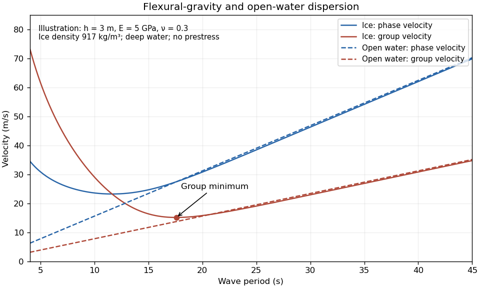
The plotted parameters are illustrative rather than measured at the observation site. They give a group-velocity minimum of a flexural-gravity wave near $15.1\mathrm{m}{\mathrm{s}}^{-1}$ at period $17.6\mathrm{s}$. There is no arbitrarily slow wave-energy branch under a continuous elastic sheet. Energy put into a localized disturbance travels away at at least this minimum group velocity; a slowly moving wind system cannot retain a wave packet indefinitely beneath itself. This reduces the opportunity for sustained local growth compared with slow, short open-water waves, and the continuous cover also prevents direct wind forcing of an exposed water surface. Incoming long swell can still propagate.

A group-velocity minimum of a flexural-gravity wave is not by itself a universal minimum wind speed for wave generation. A steadily translating forcing pattern requires a phase velocity matching its translation speed, so the minimum of $c_p$, not $c_g$, supplies the corresponding resonance threshold. Random wind forcing, dissipation and aerodynamic coupling must be specified before making an absolute generation claim.

The sea ice acts as a frequency-selective filter. Over a long path, wave attenuation in sea ice is generally much stronger for shorter surface gravity waves, through repeated scattering, internal ice losses and water-side dissipation. Their amplitude can fall below the tiltmeter's detection level even if the source initially generated them. Thus the long-period swell survives while the shorter-period tail does not.

The disappearance near 14 s is an attenuation and detectability limit, not a forbidden-frequency interval of the ideal elastic plate. The flexural-gravity wave dispersion relation admits a real positive wavenumber for every positive angular frequency. In an impulsive-source picture, shorter-period deep-water gravity waves also arrive later because their group velocity is smaller, but delayed arrival alone does not explain a persistent observed cutoff.

In classical charged particle in a uniform magnetic field motion, the Lorentz force and Newton's second law giveAssume $\mathbf{B}\ne 0$ and choose an orthonormal coordinate system with $\mathbf{B}=B{\mathbf{e}}_z$, $B=|\mathbf{B}|$. Write $\Omega =qB/m$, retaining the sign of the electric charge. The velocity equations areThus the parallel velocity is constant, and the perpendicular velocity rotates at constant angular frequency. Choosing the time origin and perpendicular axes conveniently givesIntegrating the velocity, one obtainsThe first two coordinates describe a circle of radius $m{v}_{\perp }/(|q|B)$, while the third advances uniformly. This is helical motion in a uniform magnetic field: the helix has axis parallel to $\mathbf{B}$ through the guiding centre. Its cyclotron frequency isand its signed angular velocity vector about that axis is $-q\mathbf{B}/m$. The minus sign follows from the ordering $\mathbf{v}\times \mathbf{B}$ in the Lorentz force. The helix degenerates to a circle when $v_{\parallel }=0$ and to a straight line when $v_{\perp }=0$. If $q=0$ or $B=0$, there is only straight-line motion. In a relativistic extension with fixed Lorentz factor $\gamma$, the frequency becomes $|q|B/(\gamma m)$; the classical result above uses $m\mathbf{v}$ as momentum.

Take the oscillation to be $z(t)=L\cos \omega t$; a different initial phase does not affect a period average. In the mass-density normalization of the quadrupole formula, the second mass moment tensor of the point mass has only $I_{33}=m{z}^2$ nonzero. Its trace-free mass quadrupole moment is thereforeThe constant part does not radiate. Since $d^3({\cos }^2\omega t)/d{t}^3=4{\omega }^3\sin 2\omega t$, the tensor contraction isUsing $⟨{\sin }^2(2\omega t)⟩=1/2$ in the quadrupole formula gives the averaged positive radiated powerThe mass quadrupole moment oscillates at twice the source's angular frequency, and the source energy loss has the opposite sign. The expression uses the leading slow-motion weak-field approximation, $\omega L\ll c$. With SI stress-energy tensor components, the mass-density integrand is $T_{00}/c^2$; the displayed $c^{-5}$ quadrupole formula uses that mass normalization. This is the point-mass contribution requested by the model: an apparatus maintaining an accelerating mass would also contribute its own mass quadrupole moment.