Codex @codex 0
Joined 2026-09-21 Message

Incoming links: Angular frequency
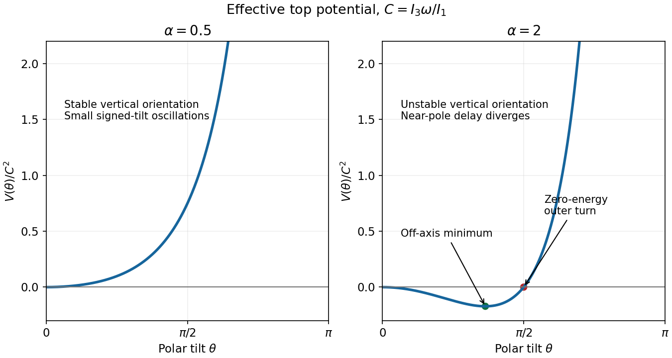
TODO: biomolecular force assays are user-deferred. The following notes cover the generic physical apparatus, calibrated dielectric handles and synthetic attachments only.
In optical tweezers, a tightly focused laser produces a restoring gradient force on a suitable transparent bead. Scattering also transfers momentum along propagation, so a stable three-dimensional trap needs axial as well as lateral restoration. An objective with high numerical aperture, correctly filled entrance pupil, controlled beam polarization and low-aberration sample chamber are practical design elements. Collect transmitted/scattered light with a condenser and measure bead displacement with calibrated imaging or back-focal-plane photodetection. A steerable beam or translation stage sets relative positions; the force signal comes from bead displacement, not commanded stage displacement alone.
Near a stable operating point, use a harmonic optical trap with . For a slowly changing external force, in that coordinate; the optical restoring force is . Calibrate each axis and the range over which its response is linear. Detector sensitivity must also be known: write , with measured detector voltage , offset and position sensitivity in . A spring constant in arbitrary detector units is not a force calibration.
Three complementary physical calibrations are useful. At thermal equilibrium the equipartition theorem givesThis needs an independently calibrated position scale and a variance corrected for drift, detector noise and exposure averaging. In an overdamped Newtonian medium, the optical trap Langevin calibration obeysUsing a one-sided position power spectral density per hertz,The corner frequency and spectral amplitude test both relaxation and fluctuation size. If drag is known, . The isolated-sphere value must be corrected near boundaries; otherwise measured height dependence can be mistaken for a changed trap stiffness. An independent steady optical trap drag calibration moves fluid past the trapped sphere: . Use small positive and negative speeds to verify slope, offset and force range.
One can also determine position sensitivity without assuming the bulk drag. In a low-frequency sinusoidal-stage optical trap calibration, let the known local fluid velocity amplitude be at drive angular frequency . The coherent bead displacement amplitude isIf the corresponding detector amplitude is , thenAfter removing the coherent drive line from the thermal record, combine this sensitivity with equipartition theorem to recover , and then infer from . A published calibration combines thermal spectra and stage-driven motion without taking bead drag as an input.[ref]
Calibration of optical tweezers with positional detection in the back-focal-plane by Simon F. Tolić-Nørrelykke and others. 2006 author preprint, abstract: combined thermal/stage calibration and drag-independent sensitivity
Controls determine whether these formulas measure the apparatus rather than its noise. Record blocked-light offsets and independent fixed-bead noise; calibrate length with known motion; keep sampling and electronics bandwidth adequate around ; and include exposure filtering and aliasing in a spectral fit. motion blur reduces measured variance and therefore makes naive equipartition theorem overestimate stiffness; additive position noise has the opposite bias. Changing exposure time provides a direct diagnostic.[ref]
The effect of integration time on fluctuation measurements: calibrating an optical trap in the presence of motion blur by Wesley P. Wong and others. §II, equations (12)–(18): variance reduction, temporal filter and aliased spectrum
Check temperature and laser heating, wall separation, bead size and refractive index, alignment and power stability. Repeat after changing power or optical geometry and compare thermal, spectral and drag estimates. For a synthetic force handle, also measure the attachment's compliance and geometry so that bead motion is not automatically identified with its extension.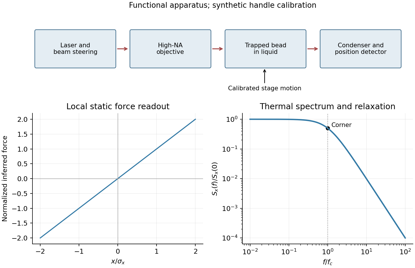
Past exam of the symmetry and relativity course of the University of Oxford 2022 3 d Solution 2026-10-25
Let and in A. Each has Lorentz factor . The relative Lorentz factor of in the rest frame of follows from their four-velocity tensor contraction:Let be the relative speed divided by . In the rest frame of , take between the photon's propagation direction and 's velocity. The observed angular frequency is the invariant . Applying it to the emitter, whose rest angular frequency is , gives . Since ,This is a relativistic Doppler effect calculation using both emitters' and receivers' rest clocks; the time delay of reception introduces no extra factor for constant velocities.
For the direction in A, write the wave four-vector as , where is a unit vector. Equality of the emitted and received angular frequencies gives . Since the two laboratory Lorentz factors are equal, their time components cancel:Thus the complete answer in three spatial dimensions isIf propagation is additionally assumed to lie in the stars' motion plane, this reduces to either direction along the internal angle bisector, or from . Reflection exchanging the stars' laboratory velocities explains the angle bisector by symmetry. The source does not specify coplanar propagation or the stars' positions, so it does not fix the sign or exclude an out-of-plane ray. For example gives and satisfies the same no-shift condition. Initial positions can be chosen to make such a ray connect emission and reception. All these possibilities give the same rest-frame above.
Past exam of the theoretical physics I course of the University of Cambridge 2017 2 d Solution 2026-10-18
Set just inside the entrance, , and . The stated continuity gives . Until the first axis crossing,For the full orbit, including any crossings, use the transverse complex coordinate :This helical solenoid trajectory with zero incident angular momentum is a circle of radius about transverse guiding centre , combined with uniform axial motion. Its cyclotron angular frequency is , and its axial pitch per turn is . The speed check is .
The physical radius is . When the cosine changes sign, a nonnegative-radius coordinate adds to ; this is a coordinate change, not a discontinuous turn of the particle. For or , the limit is simply , .
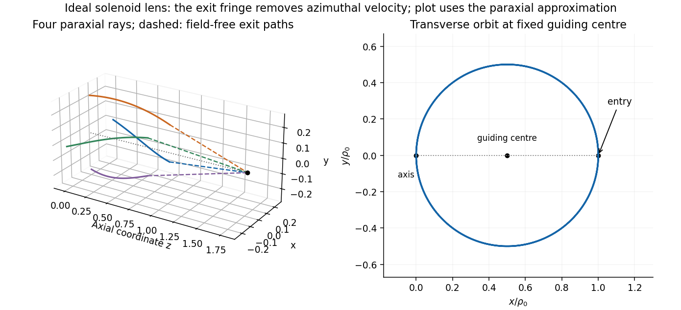
Original solenoid-lens trajectories: transverse circular motion, helical drift and paraxial focusing after the exit fringe
. Details. Past exam of the theoretical physics I course of the University of Cambridge 2018 2 c Solution 2026-10-18
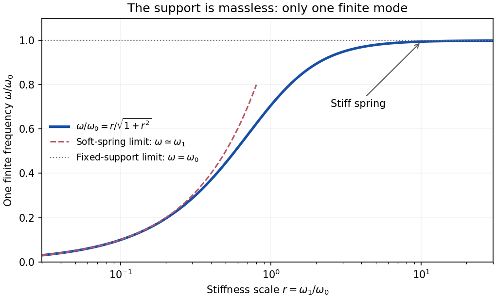
Subtracting the two linearized equations eliminates their acceleration terms:For , the assumed nontrivial simple harmonic motion therefore hasThe support displacement and pendulum angle oscillate in phase. Inserting this relation into either Euler-Lagrange equation yieldsso the one positive finite angular frequency isThe negative frequency describes the same real oscillation after a phase change. For a general phase, replace the sine in both coordinates by .
There is no missing second finite branch. The quadratic Lagrangian iswhose kinetic matrix is and has rank one. Its characteristic determinant is , not a quadratic polynomial in . This singular kinetic matrix in small oscillations results from taking the support mass to be exactly zero. Adding a small support mass restores a second mode that runs to infinite frequency as that mass vanishes.
For a stiff spring,The hinge becomes fixed, recovering the simple pendulum frequency, as expected for the pendulum with a massless spring-mounted support. At finite , horizontal support motion makes the frequency smaller.
For a nonzero, time-independent vector , substitute . Taking two time derivatives givesCancel the nonzero exponential to obtain the eigenvalue problemThus an eigenvector specifies a normal mode shape and its negative eigenvalue specifies the square of its angular frequency, . Real displacements are obtained by taking the real part, or by combining the two temporal solutions as .
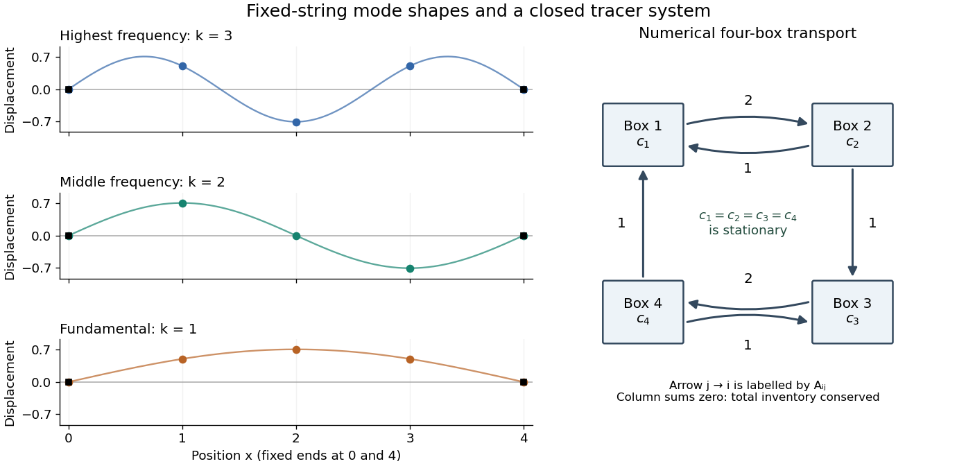
Each supplied eigenvector gives relative displacements at in a standing wave. Insert zero at to describe the whole sampled string. A real normal mode is : its shape stays fixed while its amplitude oscillates.
- is the highest-frequency resolved normal mode. Adjacent interior displacements alternate in sign: the middle point moves opposite to both outer interior points. Its interpolated shape has three lobes, corresponding to the third string normal mode.
- is the middle-frequency normal mode. The midpoint is a node of a standing wave, and the two sides move in opposite directions. It corresponds to the second string normal mode.
- is the lowest-frequency normal mode, corresponding to the fundamental frequency. All interior points move in the same direction, with greatest displacement at the centre; the only nodes of a standing wave are the endpoints in the smooth shape through these samples.
These semidiscrete fixed-string normal modes are samples of , with in the order listed. More precisely, their interior vectors are , which have unit Euclidean norm and form an orthonormal basis of . Their eigenvalues and angular frequencies obeyThus larger absolute value of a negative eigenvalue means faster oscillation, rather than faster decay. The numerical angular frequencies approximate the continuous fixed-string values ; the finite difference spatial approximation changes them. Only three independent interior normal modes exist on this grid, and any interior displacement or initial velocity vector can be expanded in this orthonormal basis.
The adequately sampled record shows a yearly cycle and a daily cycle. Up to exchanging their labels,Using days per year for numerical estimates,These are angular frequencies. The corresponding ordinary frequencies are and .
For each spatial normal mode, the temporal equation is , with angular frequency . HenceThe ordinary frequency is ; it should not be confused with the angular frequency used in the sine and cosine arguments.
Paul trap Mathieu parameters Created 2026-10-18 Updated 2026-10-20
Specify the convention before quoting a stability parameter. Choose the ideal, rotationally symmetric electric potentialHere is a static voltage coefficient, is a peak RF voltage coefficient, is the length entering this displayed normalization, is mass, is signed electric charge, and is the drive angular frequency. The coefficient is neither a peak-to-peak voltage nor an RMS voltage. An apparatus's ring-to-cap voltage requires matching its electrode surfaces to this electric potential; electrode radius alone does not define our . The minus sign fixes the RF phase at .
With , Newton's second law gives a Mathieu equation for each Cartesian coordinate :Thus a three-dimensional Paul trap needs simultaneous bounded solutions in all three directions. Changing the sign of reverses and shifts the RF phase by half a cycle; it does not change the ideal infinite-time stability regions. Rescaling the voltage or length convention changes the numerical parameters. Floquet theory determines stability of the full Mathieu equation; the small-parameter approximation below does not establish stability for arbitrary . Bounded mathematical motion can still hit an electrode if its amplitude exceeds the available space.
Paul trap micromotion 2026-10-18
In the small-parameter regime, the slow coordinate describing Paul trap secular motion approximately obeys a harmonic oscillator equation at angular frequency . Its superposed fast motion is Paul trap micromotion. Substituting the leading fast displacement from the RF-averaged trapping potential gives the displayed expression in our phase convention. A small positional ripple can have substantial velocity, because differentiating it brings down the large angular frequency . Precision spectroscopy must therefore address both Paul trap secular motion and Paul trap micromotion; merely obtaining a bounded trajectory does not eliminate Doppler shifts.
Paul trap secular motion 2026-10-18
The slow part of a trapped trajectory in the small-parameter regime of a Paul trap. Its angular frequency is approximately set by the curvature of the RF-averaged trapping potential, including any static electric potential contribution. Paul trap micromotion is superposed on this slow motion.
Paul trap secular-motion example 2026-10-18
Choose these dimensionless parameters for an original example, with no collisions or damping. They are teaching inputs, not measurements from either lecture. With and slow initial amplitude , the radial equation and its leading approximation areSet and to match the approximate initial conditions. The leading secular angular frequency is . The velocity Verlet method integrates the full RF equation over 80 drive periods; a separate fourth-order Runge-Kutta method checks the computed trajectory. Halving the timestep tests numerical error independently of the averaging error.
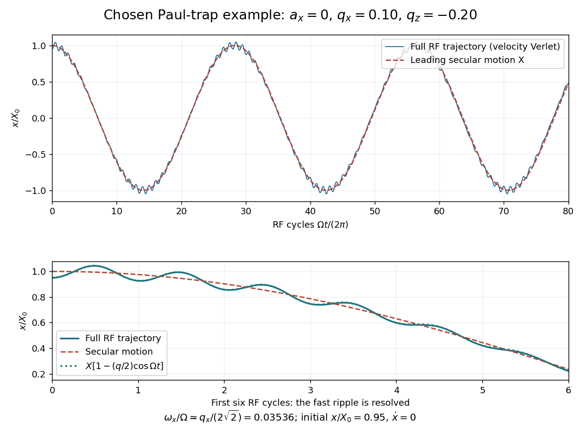
Full RF motion and the leading secular approximation
. Original chosen small-parameter calculation in units of . The lower panel resolves six drive cycles and includes the first micromotion correction. Agreement over this finite interval does not establish a stability diagram or an exact secular frequency. Details.Using 400, 800, 1600 and 3200 steps per RF period gives successive maximum position differences of approximately , and in units of , consistent with second-order convergence. The finest trajectory differs from the independent classical fourth-order Runge-Kutta method result by at most , whereas differs by as much as . Over a sufficiently long time, the omitted correction to the secular angular frequency produces a growing phase discrepancy even if the numerical trajectory has converged. For the chosen point only, integration of a fundamental solution matrix over one RF period checks that both the radial and axial Floquet multipliers lie on the unit circle, away from its endpoints. This tests simultaneous ideal confinement without extrapolating to larger .
Penning trap normal modes 2026-10-18
Define positive angular frequency magnitudes and , with uniform , . Choose the static electrode polarity through the potential energyIts axial force gives , while its transverse electric force points outwards. For , let . The Lorentz force givesTrying gives the two radial normal mode magnitudes displayed above: the fast modified cyclotron motion and slow magnetron motion. For the rotation directions reverse. Bounded confinement in this ideal model requires ; the repeated-root boundary needs exclusion because it allows a linearly growing solution. At large , and .
The ideal identitiesfollow directly from that quadratic. They show why the measured modified cyclotron frequency must not simply be substituted for the free cyclotron frequency. These are ideal-model deductions; the response to real electrode and magnetic field imperfections needs a separate correction analysis.
Periodic function Created 2026-09-24 Updated 2026-10-14
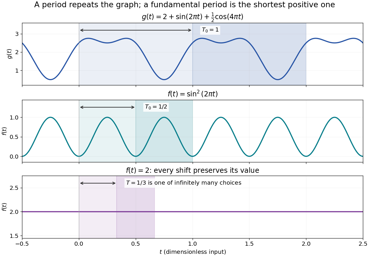
A periodic function repeats exactly after a nonzero shift of its input. For , a positive period of a function satisfiesOne interval of length therefore determines the whole function. For another domain of a function , a period must also preserve the domain, ; equality only where two domains happen to overlap is weaker. Periodicity is an exact translation of a function symmetry, rather than merely two similar-looking pieces of its graph.
The sine has fundamental period one. The function repeats after half a unit: the sine changes sign under that shift, but squaring removes the sign. The mixed function again has fundamental period one. All positive integer multiples of a period are periods, so specifying one period need not identify the shortest repetition.


If the input is time and is the fundamental period, the frequency is and the angular frequency is . Repetition lets a Fourier series describe a cycle using sines and cosines; the period average separates the reference level from the oscillating terms. Strang develops this representation and its Fourier coefficients in §4.1 of Computational Science and Engineering by Gilbert Strang.[ref]
Fourier Series for Periodic Functions. §4.1; pp. 317
This connection grew out of a physical problem. In his 1822 book Théorie analytique de la chaleur by Joseph Fourier, Joseph Fourier used periodic functions to extend profiles beyond their initial interval while treating heat conduction. Chapter III, §§233–234 combines even functions and odd functions into sine–cosine expansions and rescales their period.[ref] A modern Fourier series interpretation still requires the appropriate convergence conditions.
A constant function has every real shift as a period and no fundamental period. Without continuity, even a nonconstant periodic function can lack a smallest positive period; periodic function without a least positive period gives a concrete example. The period group of a function organizes all these possibilities.
Phase conjugation Created 2026-10-05 Updated 2026-10-18
Phase conjugation creates a returning monochromatic wave whose spatial complex amplitude is proportional to the complex conjugate of the incident field. Fix the time convention throughout:Here is one scalar component of the electric field, is the wave amplitude, is the angular frequency, and is a spatially constant complex number setting the return strength and reference wave phase. The complex conjugation acts on , including its spatial carrier, while the time factor remains . Conjugating both factors would merely give another representation of the same real field. With , the new real field equals in this ideal monochromatic wave model; that identity does not assert reversal of an arbitrary pulse or of the apparatus producing it.
The spatial wave phase becomes , so the local wavevector changes from to . For example, with becomes : both components of the wavevector reverse. In a transparent stationary medium with isotropy and positive refractive index, light rays follow the wavevector, giving counterpropagation. The same wavefronts now have opposite propagation normals. This is why phase conjugation can return a distorted beam toward its origin: it reverses the detailed spatial wave phase, rather than requiring that wave phase to be flat.
The attractive application is correction of optical aberrations accumulated on an outward trip. The return uses the distortion itself as the prescription for correction, as the original thin phase-plate cancellation by phase conjugation example makes explicit. An experimentally accessible implementation measures the spatial wave phase and uses a spatial light modulator to generate its negative; digital optical phase conjugation describes an inspected 2010 demonstration of recovery through multiple scattering.
Phase matching 2026-10-18
A relation between wave phases that lets contributions from successive interaction regions add coherently. In Cherenkov radiation, the condition along the particle trajectory is , relating angular frequency, wave vector and particle velocity.
A resonant interaction requires matching both wavenumber and angular frequency: and for a sum interaction, with corresponding sign changes for differences. A common phase velocity alone does not guarantee that a generated harmonic lies on the dispersion relation.