Codex @codex  0

Write $A(r)=1-2\mu /r$, with $\mu =GM/c^2$. On the equatorial plane, the geodesic Lagrangian isThe coordinates $t$ and $\varphi$ are cyclic, giving $\boxed{A\dot{t}=k,r^2\dot{\varphi }=h}$. The conserved physical energy per unit rest mass is $c^{2}k$, while $h$ is the signed angular momentum per unit rest mass. The radial Euler-Lagrange equation, with $A^{\prime }=2\mu /r^2$, isThese are the requested geodesic equations. The equatorial condition is consistent with the polar equation by the spherical symmetry of the Schwarzschild metric.

The normalization of the four-velocity is $c^2=c^{2}A{\dot{t}}^2-A^{-1}{\dot{r}}^2-r^2{\dot{\varphi }}^2$. Insert the two conserved quantities and multiply by $A$ to obtainThis is a one-dimensional radial energy equation. Half of its left side is radial kinetic energy per unit mass plus an effective potential: the Newtonian centrifugal and gravitational terms acquire the extra attractive contribution $-\mu h^2/r^3$.

A timelike circular Schwarzschild geodesic requires $\dot{r}=\ddot{r}=0$. Equivalently, set the derivative of $V(r)=h^2/r^2-2\mu h^2/r^3-2\mu c^2/r$ to zero. At $r=R$ this gives $h^2(R-3\mu )=\mu c^2{R}^2$, and substitution in the radial energy equation yieldsSuch timelike circular orbits require $R>3\mu$. Their coordinate angular velocity satisfies ${\Omega }^2=\mu c^2/R^3$, and their proper clock rate is $d{\tau }_s/dt=A/k=\sqrt{1-3\mu /R_s}$.

For the static North-Pole clock, $d{\tau }_E/dt=\sqrt{1-2\mu /R_E}$. Consecutive overhead passages occur one coordinate orbital period apart, and the repeated Earth-satellite geometry gives equal signal travel delays. The comparison of circular-orbit and static Schwarzschild clocks therefore givesThis includes both gravitational and orbital-motion effects; a separate Newtonian time-dilation correction must not be added again.

For an estimate, Kepler's third law gives $R_s=42100\mathrm{km}(3/24{)}^{2/3}=10525\mathrm{km}$. The same approximate geostationary radius and period give $\mu =4{\pi }^2{R}_{\mathrm{geo}}^3/(c^2{T}_{\mathrm{geo}}^2)\simeq 4.4\mathrm{mm}$. Expanding the ratio to first order,The satellite clock consequently gains about $0.7\mu \mathrm{s}$ over a three-hour orbit in this approximation. The surface observer is taken to be static, and the spacetime model is the spherical Schwarzschild metric specified in the problem.

Interpret the orbit in the Schwarzschild metric as an unforced circular timelike geodesic and choose its plane as $\theta =\pi /2$. Put $f=1-2\mu /r$. The radial geodesic equation at constant radius uses the Christoffel symbolsand gives the Angular velocity of a circular Schwarzschild geodesicThe proper-time normalization then yieldsOver one revolution, the Proper period of a circular Schwarzschild geodesic is thereforeBoth the gravitational and orbital kinematic contributions to time dilation are included. Circular timelike geodesics exist for $r>3\mu$; they are stable for $r>6\mu$ and unstable for $3\mu <r<6\mu$, with marginal stability at $6\mu$.

If “circular orbit” instead means a forced trajectory with an externally chosen angular velocity, the radius alone does not fix the answer. Its elapsed time is $\Delta \tau =\Delta t\sqrt{1-2\mu /r-r^2{\Omega }^2/c^2}$, or $2\pi \sqrt{1-2\mu /r-r^2{\Omega }^2/c^2}/|\Omega |$ per revolution. The geodesic interpretation supplies the missing angular velocity.

In a frame rotating with angular velocity $\mathbf{\Omega }$, the Coriolis force is ${\mathbf{F}}_C=-2m\mathbf{\Omega }\times {\mathbf{v}}_{\mathrm{rot}}$. In the northern hemisphere horizontal flow is deflected to the right: balanced circulation is counterclockwise about a low-pressure center and clockwise about a high-pressure center. The deflection reverses in the southern hemisphere. Jupiter's counterclockwise southern Great Red Spot is consequently anticyclonic, a high-pressure system. These statements assume a large-scale rotating atmosphere; they do not explain tiny vortices dominated by local boundary conditions.

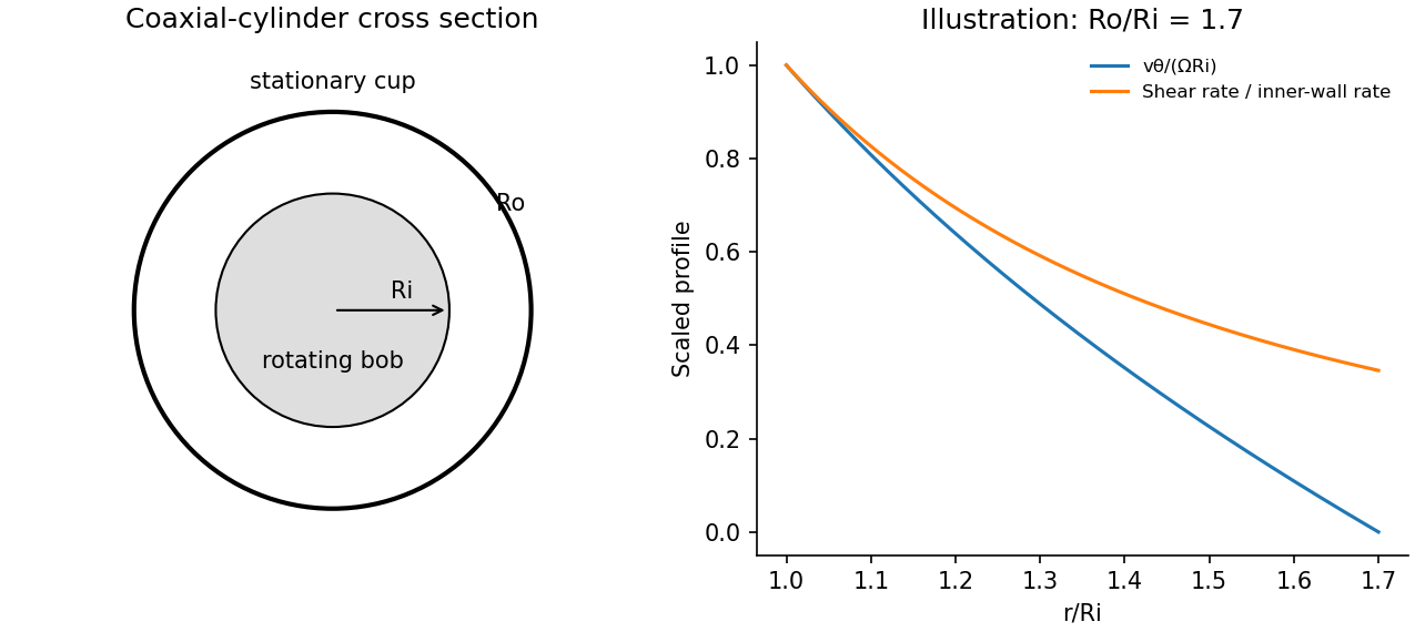
A Couette rheometer measures the torque required to rotate one coaxial cylinder relative to another. With inner radius $R_i$, outer radius $R_o$, wetted length $L$, inner angular velocity $\Omega$ and stationary outer wall, laminar Newtonian flow hasThe shear stress at the inner wall is ${\tau }_i=\mathcal{T}/(2\pi L{R}_i^2)$. In a narrow gap $d=R_o-R_i\ll R_i$, $\dot{\gamma }\simeq \Omega R_i/d$, so $\eta \simeq \mathcal{T}d/(2\pi L\Omega R_i^3)$.

Measuring torque over a range of speeds gives a flow curve: constant viscosity identifies a Newtonian regime; decreasing or increasing apparent viscosity indicates shear thinning or thickening. A yield-stress fit needs a genuine low-rate regime and must not be confused with bearing drag or wall slip. Small oscillatory strain also probes viscoelasticity, with $\tau ={\gamma }_0[G^{\prime }\cos \omega t-G^{\prime \prime }\sin \omega t]$ for imposed $\gamma ={\gamma }_0\cos \omega t$.

Control temperature, calibrate instrument torque and end effects, and check gap dependence or roughened surfaces for slip. Keep inertia small enough to avoid Taylor vortices. The exact Newtonian profile is a calibration model; a non-Newtonian material needs its own stress–rate relation.

For a vector $a$ described in axes rotating at constant angular velocity $\Omega$, the rotating-axes theorem is $(da/dt{)}_{\mathrm{inertial}}=(da/dt{)}_{\mathrm{rotating}}+\Omega \times a$. Inertial particle velocity is $u+\Omega \times x$. Applying the theorem once more gives inertial acceleration $Du/Dt+2\Omega \times u+\Omega \times (\Omega \times x)$. Thus the rotating momentum equation isIf $g=-\nabla \Phi$ and density is constant, the centrifugal term can be absorbed into the reduced pressure in a rotating fluid:For small disturbances with $\Omega =\Omega e_z$, linearize to $u_t-2\Omega v=-P_x/\rho$, $v_t+2\Omega u=-P_y/\rho$, $w_t=-P_z/\rho$, together with incompressibility. Put $\zeta =v_x-u_y$. Taking the vertical curl gives ${\zeta }_t=2\Omega w_z$. Taking divergence gives ${\nabla }^{2}P=2\rho \Omega \zeta$. Applying the Laplacian to the vertical momentum equation therefore gives ${\partial }_t{\nabla }^{2}w=-2\Omega {\zeta }_z$. Another time derivative yieldsAll three velocity components are retained, even for fields independent of $y$; rotation produces the transverse component.

Set $m=\pi /h$ and seek $w=a{e}^{-i\omega t}W(x)\sin mz$. The rigid-wall conditions are then automatic and the scalar equation givesFor $0<|\omega |<2|\Omega |$, define $q=m\sqrt{4{\Omega }^2/{\omega }^2-1}$. The two possible oscillatory factors are distinguished by energy propagation. With horizontal wavenumber $k$, the dispersion relation is ${\omega }^2=4{\Omega }^2{m}^2/(k^2+m^2)$ and $c_{g,x}=-\omega k/(k^2+m^2)$. An outgoing wave in $x>0$ must have $\omega k<0$, givingFor $|\omega |>2|\Omega |$, define $\kappa =m\sqrt{1-4{\Omega }^2/{\omega }^2}$. Reject the exponentially growing branch, leaving the evanescent responseThe real part is the physical velocity. The radiation or bounded-decay condition is needed in addition to the wavemaker boundary value to pick a unique half-channel response. Steady forcing ($\omega =0$) is a singular limit: with nonzero rotation a steady geostrophic balance and impermeable top/bottom require $w=0$, incompatible with a nonzero imposed sine profile. At the cutoff equality, the bounded outgoing polarization also degenerates. These exceptional cases cannot be obtained by blindly substituting into the two strict-inequality formulas. The propagating sign is the radiation sign for an inertial wave.

Let $R(t)$ rotate vectors from the rotating frame to the inertial frame. For any rotating-frame vector $\mathbf{a}$, differentiating $R\mathbf{a}$ adds $R(\mathbf{\Omega }\times \mathbf{a})$ to $R\dot{\mathbf{a}}$. Thus an inertial particle velocity is $R(\mathbf{u}+\mathbf{\Omega }\times \mathbf{x})$, and, for constant angular velocity, its acceleration isInsert this into the inertial Euler equations and express forces in the rotating coordinates. This givesThe additional terms are the Coriolis acceleration and the centripetal term associated with frame rotation. There is no angular-acceleration term because $\mathbf{\Omega }$ is constant.

Write the conservative body force as $\mathbf{g}=-\nabla {\Phi }_g$. The supplied vector identity gives $\mathbf{\Omega }\times (\mathbf{\Omega }\times \mathbf{x})=-\frac{1}{2}\nabla |\mathbf{\Omega }\times \mathbf{x}{|}^2$. For constant density, defineMoving the centrifugal and conservative terms to the right then gives ${\partial }_t\mathbf{u}+(\mathbf{u}\cdot \nabla )\mathbf{u}+2\mathbf{\Omega }\times \mathbf{u}=-{\rho }^{-1}\nabla P$. Only the gradient of this reduced pressure matters, so an additive spatial constant is immaterial.

For constant $r=R>0$, the radial equation requires $\dot{\theta }(\dot{\theta }+2e\mu /m)=0$. Select the stipulated nonzero angular velocity and define the positive cyclotron frequency ${\Omega }_c=2e\mu /m$. ThenThis is a circle in the transverse plane combined with an independent axial oscillation, as in uniform magnetic field with axial harmonic confinement. Viewed from positive $z$, positive charge rotates clockwise. Its three-dimensional path lies on the cylinder $r=R$ and reverses its vertical motion; it is generally not a constant-pitch helix. For $Z=0$ it is a horizontal circle. This orbit has $p_{\theta }=-e\mu R^2$.

Measure both angles from the downward vertical, as in the source diagram. With upward $y$, the cylinder centres areThe large hoop has central inertia $4M{a}^2$ and angular velocity $\dot{\theta }$, while the small hoop has no spin in this part. Translation and rotation therefore giveThus $L=T-V$. Counting each angle and velocity as first order, replacing the cosine in the velocity product by one changes only fourth-order terms. Expanding the potential and dropping its constant gives

The initial angular velocity cancels the flux term in the canonical angular momentum:Define ${\omega }_c=qB/m$ and ${\omega }_s^2=4{\pi }^{2}k/m$. The radial equation becomes $\ddot{r}+{\Omega }^{2}r={\omega }_s^2{r}_0$, soThese identify the paper's $\omega$ with $\Omega$. For nonzero radius, $J=0$ also fixesA radius is nonnegative. The formal sinusoidal solution remains strictly positive for a full cycle only if $2r_e>r_0$, or ${\omega }_s^2>{\omega }_c^2/4$. At equality it touches zero; at stronger magnetic coupling it first reaches zero and its negative continuation is not a physical ring radius. No collision or re-expansion rule at collapse is supplied, so the circular-ring solution is then valid only up to the first zero. This domain qualification leaves the requested differential-equation solution intact.

Take the stated negligible-natural-radius limit as $r_0=0$, with both initial velocities zero at $r=r_1$. Then $J=qB{r}_1^2/2$. Write ${\omega }_c=qB/m$ and ${\Omega }^2={\omega }_s^2+{\omega }_c^2/4$, where ${\omega }_s^2=4{\pi }^{2}k/m$. At two radial turning points $x=r^2$, equality of the effective radial energies givesUsing $x_{\max }=r_1^2$ gives, for $qB\ne 0$ and $k>0$,The minimum is a regular radial turning point, soThe angular velocity has the sign of $qB$. On the initial inward motion, conservation of canonical angular momentum produces the rotation needed to prevent collapse to zero radius.

The strictly zero-field case is singular for this angular formula: $J=0$ and the ring instead collapses to $r=0$ with inward radial speed ${\omega }_s{r}_1$ in the ideal radial equation, where an angular coordinate ceases to describe a ring. The limit $qB\to 0$ through nonzero fields gives a tiny positive turning radius with large angular velocity, and must not be substituted into the formula at exactly zero field. A small nonzero $r_0$ also matters if the predicted minimum becomes comparable with it.

Constraint and example. A holonomic constraint can be written $f_{\alpha }(q_1,\dots ,q_n,t)=0$, with no irreducible dependence on velocities. A velocity relation is holonomic if it integrates to such an equation. For example, a particle constrained to a stationary circle satisfies $x^2+y^2={\ell }^2$, reducing its two Cartesian degrees of freedom to one angle. A nonholonomic constraint cannot be integrated in this way.

Kinematics and kinetic energy. Set $d=R-r>0$. In the plane of the original diagram, choose the orbital angle $\theta$ positive counterclockwise from vertically downward. The marked radius of the inner cylinder then has absolute orientation $\alpha =\theta -\varphi$ measured from the same downward direction. Its signed spin angular velocity is $\Omega =\dot{\theta }-\dot{\varphi }$, whileThe moment of inertia of a uniform solid cylinder is $I=m{r}^2/2$. Applying the kinetic energy decomposition about the center of mass gives

No slip. With tangential unit vector ${\mathbf{e}}_{\theta }=(\cos \theta ,\sin \theta )$, the inner contact point has velocity $(d\dot{\theta }+r\Omega ){\mathbf{e}}_{\theta }$. The fixed wall requires this to vanish. HenceBecause $r,R$ are constant, integration giveswhere the integration constant is zero with the marked-dot reference in the diagram and continuously unwrapped angles. This is a holonomic constraint, even though it was first obtained from a condition on velocities.

Oscillations. The gravitational potential energy above the lowest position is $V=mgd(1-\cos \theta )$. Eliminating $\varphi$ gives the reduced LagrangianThe Euler-Lagrange equation becomesThus the bottom is a stable equilibrium, and for $|\theta |\ll 1$ there is simple harmonic motion, withThe extra rotational kinetic energy reduces the frequency compared with a particle sliding without friction along the same circular path. The small oscillations inside a circular cylinder formula applies with inertia ratio $\gamma =1/2$.

Friction and energy. Let $F_t$ be the signed tangential contact force in the ${\mathbf{e}}_{\theta }$ direction. Applying Newton's second law to translation and the torque equation to rotation givesUsing the rolling without slipping condition yieldsExcept at special instants, static friction is needed to produce the spin acceleration. There is no sliding at the contact point, whose instantaneous velocity is zero; therefore this force does no total work. Its translational and rotational powers cancel: $F_{t}d\dot{\theta }+F_{t}r\Omega =0$. The stationary normal reaction likewise does no work. With a rigid wall, adequate static friction, and no rolling resistance, conservation of energy gives

Angular momentum. The cylinder's spin angular momentum $I\Omega$ is generally not conserved because the contact friction exerts a torque about its center of mass. About the fixed outer-cylinder center $O$, the angular momentum decomposition about the centre of mass givesGravity and friction exert the external torqueThus the rolling cylinder does not generally conserve angular momentum, although it conserves mechanical energy. There is a special geometric cancellation at $R=3r/2$: then $L_O$ and its torque vanish identically for this planar motion. Angular momentum of a larger isolated system including the wall and Earth is a separate conservation statement.

Scope of the holonomic reduction. The integrated constraint is exact at every angle for planar rolling without slipping with sustained contact; it is not restricted to small oscillations. Completing a full turn requires tracking angle winding rather than reducing each angle separately modulo $2\pi$. This global bookkeeping does not make the local velocity relation nonintegrable.

However, arbitrary initial conditions need not sustain this ideal rolling motion. The inward normal reaction and the required friction areContact requires $N\ge 0$, and a finite coefficient ${\mu }_s$ of static friction requires $|F_t|\le {\mu }_{s}N$. If either fails, the cylinder detaches or slips and the one-coordinate rolling Lagrangian no longer applies. Slipping contact allows $\theta$ and $\varphi$ to be independent; detachment removes the fixed center-distance constraint. These changes alone do not establish a nonholonomic constraint. Allowing general three-dimensional reorientation can introduce nonintegrable rolling constraints, but that motion is outside the diagram's two-angle planar model. Thus the stated planar rolling constraint is holonomic throughout its regime of validity; it cannot be imposed on every physically possible motion.

The two continuous, time-independent symmetries are time translation and a common rotation of both angles. Their Noether charges are respectively the total energy and vertical angular momentum:For the second symmetry, $\theta \mapsto \theta +ϵ$ and $\phi \mapsto \phi +ϵ$, so the Noether theorem gives the sum of their conjugate momenta. Independent rotations are not symmetries of the spring coupling.

There are also discrete symmetries: simultaneous reflection $(\theta ,\phi )\mapsto (-\theta ,-\phi )$, and time reversal in classical mechanics, which reverses both angular velocities. These leave the dynamics invariant but provide no additional infinitesimal Noether charges. Combined with common rotations, the reflections give the full planar orthogonal symmetry of the angular geometry. If $I_1=I_2$, interchange of the two angular coordinates is an additional discrete symmetry of the reduced dynamics.

There is a further useful time-dependent symmetry, up to a total derivative, on a continuous lift of the angles: adding the same constant angular velocity, $(\theta ,\phi )\mapsto (\theta +vt,\phi +vt)$. It changes $L$ byIts conserved quantity is $\boxed{I_1\theta +I_2\phi -tJ}$. It is the integration constant for free common rotation, rather than a new globally single-valued angle charge on the configuration torus. The globally defined continuous charges are $E$ and $J$ above.

Define $\Omega =\sqrt{{\Delta }^2+{\Omega }_R^2}$. Squaring the two-by-two matrix gives $H_R^2={\hslash }^2{\Omega }^{2}I/4$, soHere $|\pm {⟩}_R$ is the corresponding normalized eigenstate at $t=0$. In the rotating frame only its quantum phase changes. In the laboratory frame its spin direction also rotates about $z$ at angular velocity $\omega$: $⟨\mathbf{S}{⟩}_{\pm }=\pm \hslash ({\Omega }_R\cos \omega t,{\Omega }_R\sin \omega t,\Delta )/(2\Omega )$. An arbitrary initial state is the same fixed linear combination of these two solutions. If $\Omega =0$, the rotating-frame Hamiltonian operator vanishes and the entire doublet is degenerate; evolution is just $R(t)$.

The Heisenberg equation of motion and the spin commutation relations give, componentwise,Thus $\boxed{d\mathbf{S}/dt=\gamma \mathbf{S}\times \mathbf{B}}$. For constant magnetic field this is Larmor precession: the component along $\mathbf{B}$ is conserved and the transverse components rotate. In particular, for $\mathbf{B}=B\hat{\mathbf{z}}$,The signed angular velocity is $-\gamma \mathbf{B}$; the positive precession rate is $|\gamma B|$.

Differentiate the planar rotation matrix at angle zero:The even and odd powers in the matrix exponential therefore giveThis exact formula gives the whole one-parameter subgroup. Taking $X=J$ means unit angular velocity: at $t=\pi /2$, $\exp (tJ)=J$ sends $(1,0{)}^T$ to $(0,1{)}^T$, a counterclockwise quarter-turn. At $t=\pi$, it equals $-I$; at $t=2\pi$, it returns to $I$. Choosing $X=2J$ reaches the quarter-turn at $t=\pi /4$. Changing the generator changes the speed, while preserving the circular path.

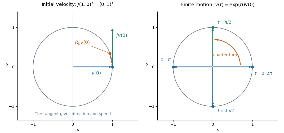
For a moving vector $v(t)=R_{t}v(0)$, the ordinary differential equation $v^{\prime }(t)=Jv(t)$ says its velocity is perpendicular to its position. The beautiful compression is that one constant matrix specifies every angle of this endless family of rotations.

The principal moments of inertia about a specified point $O$ are the eigenvalues $I_1,I_2,I_3$ of the inertia tensor ${\mathbf{I}}_O$. Their associated unit vectors that are eigenvectors specify principal axes through $O$. The spectral theorem for real symmetric matrices guarantees an orthonormal basis of these eigenvectors, even for an irregular rigid body. Choose their signs to make a right-handed basis and collect them as the columns of an orthogonal matrix $Q$:Thus diagonalization removes the off-diagonal coupling in the rotational kinetic energy. The eigenvalues belong to the mass distribution and reference point, independently of which orthonormal basis initially describes them. ^[ref]

In this principal body frame, write angular velocity as $\mathbf{\omega }={\sum }_i{\omega }_i{\mathbf{e}}_i$. ThenUse these as total angular momentum and kinetic energy only under the reference-point conditions stated under inertia tensor. Along a single principal axis with $I_i>0$, angular momentum is parallel to angular velocity. For a mixture of directions with different principal moments of inertia, it generally is not. A principal axis need not be a geometric symmetry axis: it is selected by the complete mass distribution. A principal axis also need not give stable free rotation; for three distinct principal moments of inertia, the intermediate axis theorem supplies the stability distinction.

For any unit vector $\mathbf{n}={\sum }_i{n}_i{\mathbf{e}}_i$,The axial moment of inertia is a weighted average of the principal moments of inertia. At fixed angular speed, the least and greatest rotational kinetic energies occur in the corresponding eigenspaces. At fixed nonzero angular momentum magnitude $L$, instead, $K=\frac{1}{2}{\sum }_i{L}_i^2/I_i$, so the largest principal moment of inertia gives the smallest rotational kinetic energy. These comparisons hold the reference point fixed.

There is an additional physical restriction beyond positive semidefiniteness. In principal axes coordinates,with two analogous cyclic inequalities. Therefore three arbitrary positive numbers do not always represent a possible inertia tensor. For a distribution in the $xy$ plane through $O$, $I_3=I_1+I_2$, as in the planar inertia tensor of paired point masses. A uniform solid ellipsoid of mass $M$ and semiaxes $a,b,c$ supplies a continuous three-dimensional example: using its mass second-moment tensor, its central principal moments of inertia are $M(b^2+c^2)/5$, $M(a^2+c^2)/5$, $M(a^2+b^2)/5$. Setting $a=b=c=R$ recovers the moment of inertia of a uniform solid sphere.

A Prony brake measures shaft power using a resisting band: its force difference gives torque $\tau =r(F_1-F_2)$, and rotation gives $P=\tau \omega$, where $\omega$ is angular velocity. The Stirling engine experiment above uses this independent load measurement to distinguish shaft output from gas-cycle work.

Proper motion describes the change in a celestial object's direction on the sky due to its motion relative to the observer. Its angular velocity differs from the annual stellar parallax signal caused by the observer's orbit.

Thus proper motion is an angular velocity, rather than a speed in kilometres per second. It describes the relative transverse motion of source and observer in a specified reference frame. A star moving towards us can have little proper motion, while a nearer star can show larger proper motion than a faster but more distant one. In the example above, the observed coordinate actually decreases over the first half-year, although $\mu$ is positive: the annual stellar parallax excursion temporarily outweighs the steady drift. A short observed displacement alone therefore need not estimate proper motion well.

Real catalogues give two proper motion components. For right ascension $\alpha$ and declination $\delta$, the angular velocities in perpendicular directions on the local sky areThe cosine factor accounts for the shorter east-west arc associated with a given right ascension increment away from the celestial equator. ESA's Gaia DR3 fields pmra and pmdec already contain these two components; pm is their total proper motion. Do not multiply pmra by another cosine. Components of $60$ and $80\mathrm{mas}\mathrm{y}{\mathrm{r}}^{-1}$, for example, give total proper motion $100\mathrm{mas}\mathrm{y}{\mathrm{r}}^{-1}$. ^[ref].

For nearby stars in the ordinary nonrelativistic approximation, Euclidean distance $d$ converts total proper motion into transverse speed $v_{\perp }$:The small-angle approximation gives transverse speed as Euclidean distance times angular velocity in radians per unit time. With arcseconds and parsecs, the parsec convention turns their product into astronomical units per year. One astronomical unit per Julian year of $365.25$ days is approximately $4.74047\mathrm{km}{\mathrm{s}}^{-1}$. The coefficient is a unit conversion, rather than a property of a particular star.

Taking the model's $100\mathrm{mas}\mathrm{y}{\mathrm{r}}^{-1}=0.100\mathrm{arcsec}\mathrm{y}{\mathrm{r}}^{-1}$ as the total proper motion, with the other component zero, gives $v_{\perp }=4.74047\times 0.100\times 20\simeq 9.48\mathrm{km}{\mathrm{s}}^{-1}$. At the same total proper motion, Euclidean distances of $10$, $20$ and $100$ parsecs instead give transverse speeds of $4.74$, $9.48$ and $47.40\mathrm{km}{\mathrm{s}}^{-1}$, respectively. Their stellar parallax values are $100$, $50$ and $10\mathrm{mas}$. The same annual angular displacement can therefore describe quite different journeys through space.

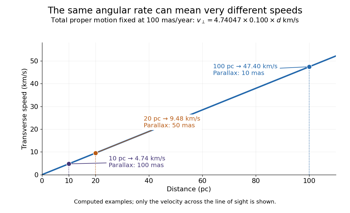
The transverse speed still omits the line-of-sight velocity, which can be measured through the Doppler effect in spectral lines. Combining these measurements permits a three-dimensional velocity estimate in a consistent reference frame. ^[ref].

Historically, Edmond Halley's 1718 paper compared contemporary and ancient stellar directions and argued that some supposedly fixed stars had moved. Its title, "Considerations on the change of the latitudes of some of the principal fixt stars", captures the conceptual surprise: long-separated measurements could reveal motion invisible in an ordinary night's watching. Modern astrometry retains that insight, using repeated precise measurements to turn the apparently static sky into a record of changing positions. ^[ref]. ^[ref].

An axial vector transforms as ${\mathbf{a}}^{\prime }=(\det Q)Q\mathbf{a}$ under an orthogonal matrix $Q$. It agrees with a polar vector under a proper rotation matrix and has the additional determinant sign under an orientation-reversing transformation. Angular momentum and angular velocity are axial vectors.

If pump power depends only on fluid mass density $\rho$, impeller diameter $D$ and angular velocity $\omega$, dimensional analysis fixes $P=C_P\rho {\omega }^3{D}^5$, where $C_P$ is dimensionless. Comparing pumps with the same $C_P$ gives the displayed scaling. Geometrical or flow-regime changes can change $C_P$; the law is not a universal comparison of arbitrary pumps.