Codex @codex  0

The mole is the SI base unit of amount of substance. One mole contains exactly $6.02214076\times 10^{23}$ specified entities, as fixed by the Avogadro constant. It counts entities rather than a fixed mass or volume. ^[ref]

A monodisperse particle suspension has a narrow distribution of particle sizes. Treating its particles as having a single radius simplifies the Perrin sedimentation experiment model; residual size variation can still affect the inferred Avogadro constant.

Full dissociation gives bulk concentrations in $\mathrm{mM}$ of $155$ for sodium, $5$ for potassium, $2$ for calcium, $114$ for chloride, and $25$ for hydrogen phosphate. The positive and negative charge concentrations are both $164\mathrm{mM}$, so the bulk is electrically neutral. At $T=298.15\mathrm{K}$,The Boltzmann distribution then givesFor completeness the coion concentrations are $114e^{-\nu }=6.65196\mathrm{mM}$ and $25e^{-2\nu }=0.0851195\mathrm{mM}$. They are depleted, not zero. Using $1\mathrm{mM}=1\mathrm{mol}{\mathrm{m}}^{-3}$ and multiplying molar concentrations by the Avogadro constant in the Grahame equation givesThis calculation retains every species. Since $|{\varphi }_0|/V_T=2.84$, a linear Debye–Hückel approximation is not justified. The large accumulation, especially of divalent counterions, follows from the valence in the Boltzmann factor. However, multi-molar local concentrations also warn that point-ion mean-field theory neglects finite ion size, hydration, specific adsorption, correlations, and changes in local permittivity. These are predictions of the stated idealized model, not precise measured interfacial concentrations.

Using $M_{\mathrm{Au}}\simeq 196.97\mathrm{g}\mathrm{mo}{\mathrm{l}}^{-1}$ and the Avogadro constant, the areal atom count isOne atom occupies each square cell of area $a^2$, so the inferred square lattice spacing isThis uses the given deposited mass and the assumed single square layer; it does not substitute a bulk gold lattice parameter for the measured areal count.

Treat each species as a dilute classical ideal gas: molecules of the same species are indistinguishable, while different species are distinguishable. Let $N_i$ be the number of molecules of species $i$, $q_i(T,V)$ its molecular partition function with energies measured from a chosen internal reference, and ${\epsilon }^{0,i}$ that reference energy per molecule relative to a common chemical energy convention. Then the mixture's canonical partition function factorizes:The $N_i!$ corrects the overcounting of indistinguishable particles. The exponential restores the species-dependent reference energies that matter for reactions. Thus the Helmholtz free energy isUsing Stirling's approximation, $\ln (N_i!)\simeq N_i\ln N_i-N_i$, and differentiating at fixed $T,V,N_{j\ne i}$ yieldsThe ideal-gas $q_i$ does not depend on the number of molecules, so no additional $\partial q_i/\partial N_i$ term appears. These are chemical potentials per molecule; multiply by the Avogadro constant for a molar chemical potential. The result assumes the thermodynamic, nondegenerate-gas limit.

For forward and reverse elementary reactions at equilibrium, the two rates are equal. Both directions have two reactant particles and use the same concentration convention, so the conversion factors cancel and $K_{\mathrm{eq}}=k_3/k_{-3}$. ThereforeFor molar rather than molecular number concentration, the bimolecular rate constant is multiplied by the Avogadro constant:Only one factor is needed: converting the two concentration factors contributes $N_A^2$, while converting the production rate from molecules to moles removes one factor.

For the conventional body-centred cubic lattice, the crystal basis structure factor of identical atoms isIt vanishes for odd $h+k+l$ and equals $2f_{\mathrm{W}}$ for even $h+k+l$. Thus the first powder diffraction ring is the $\{110\}$ family, with interplanar spacing $d_{110}=a/\sqrt{2}$.

The measured deflection is the angle between incident and scattered rays, $2\theta =40.26^{\circ }$, so the Bragg angle is $\theta =20.13^{\circ }$. Using first-order Bragg diffraction, $2d\sin \theta =\lambda$, givesThe mass density follows from two atoms per conventional unit cell, with molar mass $M=0.1838\mathrm{kg}\mathrm{mo}{\mathrm{l}}^{-1}$ and Avogadro constant $N_A$:Using $40.26^{\circ }$ as the Bragg angle would confuse $\theta$ with $2\theta$ and give an incorrect lattice constant and mass density.

In weak magnetic field and the regime of paramagnetism, localized magnetic moments with total angular momentum $J$ and Landé g-factor $\tilde{g}$ have SI volume magnetic susceptibilitywithin the Curie–Weiss law. Here $n_m$ counts magnetic ions per volume, ${\mu }_0$ is the vacuum permeability, ${\mu }_B$ is the Bohr magneton, and $\Theta$ is the Weiss temperature. The factor $J(J+1)/3$ is the zero-field average of the squared angular projection over $m_J=-J,\dots ,J$.

For one magnetic ion per formula unit, a molar volume $V_m$ contains $N_A$ magnetic ions, where $N_A$ is the Avogadro constant. Consequently $n_m{V}_m=N_A$, and the molar magnetic susceptibility isDefining the dimensionless effective paramagnetic moment $m_{\mathrm{eff}}$ by ${\mu }_{\mathrm{eff}}=m_{\mathrm{eff}}{\mu }_B$, numerical substitution givesThe normalization is per mole of formula units, which here also means per mole of magnetic ions.

The cobalt-60 mass is approximately $5.73\times 10^{-8}\mathrm{kg}$. The nuclear decay constant follows from the half-life, using a $365.25$-day year:Since radioactive activity is $A=\lambda N$, the parent population at certification isConvert the supplied atomic mass into molar mass, $M=0.05993382\mathrm{kg}\mathrm{mo}{\mathrm{l}}^{-1}$, and use the Avogadro constant:This is about $57.3\mu \mathrm{g}$ of the specified isotope. It is not the total mass of the pellets or capsule, which can also contain other material.

Dating principle. Atmospheric cosmic rays produce secondary neutrons, which can generate carbon-14 through ${}^{14}\mathrm{N}(n,p){}^{14}\mathrm{C}$. Carbon then enters atmospheric carbon dioxide and living organisms. While an organism exchanges carbon with its environment, its carbon-14 to carbon-12 ratio approximately tracks that reservoir. After exchange stops, surviving carbon-14 undergoes beta-minus decay, whereas the stable carbon remains. On the closed-sample, constant-initial-ratio model, radioactive decay givesThus radiocarbon dating infers elapsed time from the loss of an isotope ratio or of radioactive activity per fixed carbon mass. It dates cessation of carbon exchange, which need not equal the date an object was manufactured or buried. Actual calendar dating also requires radiocarbon calibration and control of contamination and reservoir differences.

Mean lifetime. For exponential decay, the half-life obeys $e^{-\lambda T_{1/2}}=1/2$, while the mean lifetime is $\tau =1/\lambda$. HenceUsing $1\mathrm{yr}=365.25\times 86400\mathrm{s}$ gives $\lambda =3.83325\times 10^{-12}{\mathrm{s}}^{-1}$ and $\tau =2.60875\times 10^{11}\mathrm{s}$.

The mass minimum and beta stability. Treat the supplied masses as nuclear rest energies in $\mathrm{MeV}$, and omit nuclear pairing as instructed. At fixed mass number $A$, the volume and surface terms of the semi-empirical mass formula are constant. Expanding the remaining terms gives a convex nuclear mass parabola,The continuous minimum in atomic number is thereforeAt $A=14$, the quadratic coefficient is $7.01302\mathrm{MeV}$ and $Z_{\ast }=6.79450$. The nearest integer is $Z=7$; the nuclear isobar of minimum mass is nitrogen-14. Maximizing nuclear binding energy alone would omit the neutron-proton rest-mass difference; its continuous optimum is slightly different, but also selects integer $Z=7$ here.

The values most useful for checking neighboring decay thresholds areConsequently carbon-14 can lower its nuclear mass by changing a neutron into a proton:For bare nuclear masses, the Q value must include the emitted electron mass. Taking $m_e{c}^2=0.511\mathrm{MeV}$,The opposite proton-to-neutron conversion would lead to $Z=5$, whose nuclear mass is $18.1567\mathrm{MeV}$ higher than that of carbon-14. Neither beta-plus decay nor electron capture can bridge that gap by supplying an electron-mass correction. For the nitrogen-14 daughter, both neighboring nuclear masses are higher: $Z=6$ by $4.13070\mathrm{MeV}$ and $Z=8$ by $9.89535\mathrm{MeV}$. Even electron capture to $Z=6$ has $Q=0.511-4.13070<0$. Thus the daughter has no further energetically allowed single beta decay in this model; physical nitrogen-14 is stable.

These threshold numbers belong to the supplied smooth semi-empirical mass formula, not to an accurate prediction of the carbon-14 electron spectrum or its long half-life. Semi-empirical mass errors can change beta-decay thresholds. Also, the instruction to omit nuclear pairing is a model simplification: even $A=14$ does not make physical pairing vanish, and even-even carbon and odd-odd nitrogen need not have the same pairing correction. No omitted pairing coefficient is guessed here.

Activity of modern carbon. Neglect the small contribution of other stable carbon isotopes when counting atoms in a gram. The Avogadro constant givesThe expected radioactive activity of that one gram isor approximately $15.0$ decays per minute per gram of carbon. A becquerel is one decay per second; the normalization is per gram of carbon, rather than per gram of the entire organic sample.

Artefact age. Its remaining activity fraction is $0.13/0.25008=0.51983$. Inverting the exponential decay law,This is the radiocarbon age on the supplied constant-initial-activity, $5730$-year half-life model. It is not a calibrated calendar date; the sample's historical initial ratio and any later carbon exchange are not supplied.

For fixed electron number $N$, the specified electron degeneracy pressure scales as $P\propto V^{-5/3}$. Differentiating at fixed low temperature gives the degeneracy-pressure bulk modulus,A monovalent sample has one conduction electron per atom. Its carrier density isusing the Avogadro constant $N_A=6.02214076\times 10^{23}\mathrm{mo}{\mathrm{l}}^{-1}$. Substitution with reduced Planck constant $\hslash =1.05457\times 10^{-34}\mathrm{J}\mathrm{s}$ and electron mass $m_e=9.10938\times 10^{-31}\mathrm{kg}$ givesEquivalently, $P=2n{E}_F/5$ and $K_T=2n{E}_F/3$ for this free electron model. This is the assumed electronic contribution, not a calculation of the complete equation of state of real potassium: ionic cohesion and interaction corrections have been excluded as instructed. The supplied pressure is the zero-temperature form, appropriate to leading order for $T\ll T_F$.

Under the one-carrier Drude model, the magnitude of the Hall coefficient gives an effective carrier densityConvert the material mass density to $1850\mathrm{kg}{\mathrm{m}}^{-3}$ and its molar mass to $0.009\mathrm{kg}\mathrm{mo}{\mathrm{l}}^{-1}$. The atomic number density isHere $N_A=6.02214076\times 10^{23}\mathrm{mo}{\mathrm{l}}^{-1}$ is the Avogadro constant. The positive Hall coefficient gives a hole-like response in a one-carrier interpretation. The Hall carrier count versus valence distinction matters: beryllium has two valence electrons, but the result is neither two free electrons nor a literal fractional atom donating charge. Its energy bands and Fermi surface invalidate the simple isotropic one-carrier inference. Electron-like and hole-like contributions with different charge carrier mobilities can yield this sign and effective count.

Treat sodium as monovalent, with one mobile electron per atom. Its mass density is ${\rho }_m=0.97\mathrm{g}\mathrm{c}{\mathrm{m}}^{-3}=970\mathrm{kg}{\mathrm{m}}^{-3}$, and its molar mass is $M=0.023\mathrm{kg}\mathrm{mo}{\mathrm{l}}^{-1}$. Using the Avogadro constant,The electron mobility $\mu =e\tau /m_e$ relates the magnitude of drift velocity to electric field. The Drude model then givesUsing $m_e=9.109\times 10^{-31}\mathrm{kg}$,The inferred time is the momentum relaxation time. Identifying it with the mean time between collisions is the intended simple isotropic Drude model assumption; small-angle scattering need not relax directed momentum in a single event.

Temperature as an equilibrium relation. Classical thermodynamics begins with the zeroth law of thermodynamics: thermal equilibrium is transitive. A thermometer can therefore assign a common empirical temperature to systems in mutual thermal equilibrium. Different thermometer properties initially give different monotone empirical scales; a resistance reading by itself does not define the absolute scale.

The Second law of thermodynamics provides a substance-independent thermodynamic scale. A reversible engine operating between reservoirs has a heat ratio depending only on their temperatures. One chooses absolute temperature so that $Q_h/Q_c=T_h/T_c$, with $Q_h,Q_c$ the positive heat magnitudes. Its reversible efficiency is $1-T_c/T_h$. Equivalently, reversible heat defines entropy through $dS=\delta Q_{\mathrm{rev}}/T$. For an equilibrium simple compressible system,Classical thermodynamics uses this relation without needing a microscopic account of entropy. A dilute-gas thermometer realizes an empirical scale approaching the thermodynamic scale after corrections for nonideal behavior.

Statistical meaning of the same derivative. In the microcanonical description, an equilibrium energy shell containing $\Omega (U,V,N)$ accessible states has $S=k_B\ln \Omega$. Its statistical temperature is consequentlyTo see why this is an equilibrium temperature, let two weakly coupled systems exchange a small energy while their total energy stays fixed. The combined multiplicity is ${\Omega }_A(U_A){\Omega }_B(U_{\mathrm{tot}}-U_A)$. Maximizing its logarithm giveswhich is equality of the two inverse temperatures. Stability requires the total entropy maximum, not only stationarity. The overwhelmingly dominant macrostate in a large system therefore realizes the thermodynamic equilibrium condition.

A large reservoir gives a small subsystem the canonical probabilities $p_i\propto e^{-\beta E_i}$, with $\beta =1/(k_{B}T)$. In that ensemble, $F=-k_{B}T\ln Z$ and $S=-k_B{\sum }_i{p}_i\ln p_i$ agree with macroscopic thermodynamic relations in their usual equilibrium regime. The equipartition identity for a classical dilute monatomic gas, $⟨p^2/(2m)⟩=3k_{B}T/2$, is a useful operational connection between microscopic motion and temperature, but is not a universal definition: quantum modes need not obey equipartition, and a system away from equilibrium need not have one temperature at all.

For finite systems one must specify the entropy convention and energy resolution; surface and fluctuation corrections can distinguish definitions that agree in the ordinary thermodynamic limit. Bounded-energy population-inverted systems can also have a negative entropy derivative and hence a negative statistical temperature. That possibility lies outside an ordinary positive-temperature ideal-gas thermometer; it does not mean temperature is merely an arbitrary average kinetic energy.

Obtaining the energy–temperature conversion. The Boltzmann constant connects entropy measured in $\mathrm{J}{\mathrm{K}}^{-1}$ with the dimensionless logarithm of a state count. Historically it could be determined from the ideal gas law $pV=N{k}_{B}T$: measure the molar gas constant $R$ and independently determine the Avogadro constant $N_A$, then obtain $k_B=R/N_A$. The independent particle-number determination matters; using $R$ alone would not fix energy per particle.

An electrical method uses Johnson-Nyquist noise. A resistor of resistance $R_e$ at known temperature has, in the classical range $hf\ll k_{B}T$, a one-sided open-circuit voltage-noise spectrum $S_V(f)=4k_{B}T{R}_e$. Over a calibrated flat bandwidth $\Delta f$,A practical measurement uses an equilibrium resistor, a calibrated low-noise amplifier and a known transfer function, subtracts or independently characterizes amplifier noise, and replaces a nominal bandwidth by the actual effective noise bandwidth. Varying temperature and fitting the mean-square voltage is more informative than treating one amplified voltage sample as the thermal variance. Other primary methods relate temperature to sound speed in a dilute gas or to calibrated particle diffusion and mobility.

There is a historically relevant unit-definition qualification: by the date of this exam, the revised SI had already taken effect on 20 May 2019. The kelvin is now defined by fixingThe same experiments now realize or compare thermodynamic temperatures using this fixed constant, whereas historically they measured the conversion constant on an independently defined temperature scale. The physical distinction between equilibrium temperature and microscopic state counting is unchanged.^[ref]

Define the positive mass collision stopping power as $S_{\mathrm{col}}/\rho =-(1/\rho )dT/dx$. For a projectile of charge $ze$, mass $M\gg m_e$, speed $v=\beta c$ and Lorentz factor $\Gamma =(1-{\beta }^2{)}^{-1/2}$, the Bethe stopping formula can be writtenHere $Z$ is the absorber atomic number, $A$ its molar mass, $I$ its mean excitation energy, $r_e=e^2/(4\pi {ϵ}_0{m}_e{c}^2)$, and $N_A$ the Avogadro constant. AlsoThe optional $\delta$ and $C/Z$ represent density and shell corrections. For a very heavy projectile $T_{\max }\simeq 2m_e{c}^2{\beta }^2{\Gamma }^2$, and the bracket reduces to $\ln (2m_e{c}^2{\beta }^2{\Gamma }^2/I)-{\beta }^2$ when those corrections are neglected. If $T$ denotes remaining projectile kinetic energy, the printed $dT/(\rho dx)$ is negative; the conventional positive stopping power has the minus sign above.^[ref]

Use number concentrations and write the electrochemical potential of a sodium ion as $\tilde{\mu }={\mu }^{\circ }+k_{\mathrm{B}}T\ln c+e\psi$. Define the inward sodium-motive force as available work per positive charge for transport from outside to inside. With $V_m={\psi }_i-{\psi }_o$,Its negative is the signed inward free-energy cost per charge; stating this direction removes a common sign ambiguity.

Long-open sodium channels establish electrochemical equilibrium, $k_{\mathrm{B}}T\ln (c_{i0}/c_o)+e{V}_{m0}=0$. This does not generally require equal concentrations: impermeant counterions can support a nonzero equilibrium membrane potential. Let $n_0=c_{i0}V$. For a large fixed-concentration external reservoir, after pumping $n$ ions out, $c_i(n)=(n_0-n)/V$ and $V_m(n)=V_{m0}-ne/C$. The sodium export cost from a capacitive vesicle for exporting another ion isThe initial-equilibrium relation was used in the last step. The first term is the incremental electrical cost and the second is the change in chemical cost from their initial balanced values.

If the intended initial reference is uncharged with $V_{m0}=0$ and $c_{i0}=c_o$, then $n_0=c_{o}V$ and the requested form in the listed variables isThat equal-concentration reference is an additional assumption. For example, $c_{i0}=2c_o$ and $V_{m0}=-(k_{\mathrm{B}}T/e)\ln 2$ also give zero initial sodium flux, but a different ion inventory. Thus the open-channel condition alone cannot determine $n_0$ from $c_{o}V$. If concentrations are molar rather than number densities, use the corresponding Avogadro constant conversion and $RT$ for molar free energies. Treating the capacitor charge discretely gives a charging-energy increment $(n+1/2)e^2/C$ rather than the differential $n{e}^2/C$; the distinction is negligible for the thousands of ions used next.

The polymer overlap concentration is reached when there is roughly one chain per coil volume. If $M$ is the chain molar mass, choose the explicit geometric convention $V_{\mathrm{coil}}=4\pi R_g^3/3$, where $R_g$ is the radius of gyration. ThenHere $c^{\ast }$ is mass per solution volume and $N_A$ is the Avogadro constant. A good solvent gives $R_g\propto N^{\nu }$ with $\nu \simeq 0.588$, approximated by $3/5$ in the Flory approximation. With a polystyrene repeat-unit molar mass of about $104.15\mathrm{g}\mathrm{mo}{\mathrm{l}}^{-1}$, the chain has approximately $N=960$ repeat units. This fixes the chain length but not the size amplitude: the problem supplies no statistical segment length or measured coil size.

For a numerical estimate, use the good-solvent size calibration for polystyrene,This empirical calibration is quoted for benzene or toluene near room temperature at molar masses above $2\times 10^5\mathrm{g}\mathrm{mo}{\mathrm{l}}^{-1}$; using it here is a modest extrapolation to $M=10^5\mathrm{g}\mathrm{mo}{\mathrm{l}}^{-1}$. It gives $R_g\simeq 11.3\mathrm{nm}$. ThusThe unrounded calibration gives about $27\mathrm{g}{\mathrm{L}}^{-1}$. This is an estimate under a stated extra material input, not a unique number determined solely by molecular weight and the phrase good solvent. Choosing a different coil-volume convention changes its prefactor. The robust chain-length dependence is $c^{\ast }\propto M^{1-3\nu }\simeq M^{-4/5}$ for a flexible good-solvent coil.

The bookkeeping reaction isBoth mass number and electric charge are conserved: $236=92+140+4$ and $92=37+55$. Express each atomic mass as the sum of its constituent rest masses minus its nuclear binding energy. The total constituent masses, including the atomic-electron masses, cancel between the two sides. Neglecting incident-neutron kinetic energy, the Q value is thereforeThe relevant initial binding is that of uranium-235. Introducing uranium-236 as an intermediate state is possible only if the neutron-capture energy is also accounted for.

In the stated coefficient convention,Uranium-235 has odd $A$, hence ${\delta }_B=0$. Both products are odd–odd: rubidium has $(Z,N)=(37,55)$ and caesium has $(55,85)$. Each therefore has ${\delta }_B=-12/\sqrt{A}$ MeV. Direct substitution givesThis is the estimate from the supplied smooth mass formula, rather than a value imported from measured isotope masses.

For $100$ MW recovered as the stated fission energy, the annual energy output is $10^8(365.25)(86400)$ J. ThusEach event consumes one uranium-235 atom. With Avogadro constant $N_A=6.02214076\times 10^{23}$ mol${}^{-1}$ and molar mass approximated as $235$ g mol${}^{-1}$,This uses the stated power directly as recovered fission power; an unspecified conversion efficiency or additional heat-loss correction cannot be inferred from it.

A colloidal grain in a liquid is large enough to see with a microscope, yet small enough for thermal motion to compete with its tendency to settle. In the Perrin sedimentation experiment, the equilibrium number density falls with height: a visible miniature atmosphere. Counting grains at different heights measures an energy scale; tracking their Brownian motion measures a transport rate. Connecting both to the same Avogadro constant makes the experiment a quantitative test of kinetic theory. The Wiener measure describes an idealized path law; these measurements instead test a physical model and its material parameters.

Jean Baptiste Perrin's 1909 memoir traces his sedimentation experiments to May 1908. It reports relative counts $100$, $47$, $22.6$, $12$ at heights $5$, $35$, $65$, $95\mu \mathrm{m}$, and compares radius estimates from Stokes settling velocity, counted grain mass, and rows of touching grains.^[ref]

The 1926 lecture describes resin precipitated from alcohol into water, washed and fractionated by centrifugation to obtain nearly monodisperse gamboge or mastic grains. Diameter and density were measured separately. A sealed slide-and-cover-glass chamber prevented evaporation; a vertical microscope resolved roughly $2\mu \mathrm{m}$ layers through a roughly $0.1\mathrm{mm}$ depth. Refocusing and photographing compared layer populations after equilibrium; changing temperature reversibly changed the distribution.^[ref]

In Les Atomes (1913), Jean Baptiste Perrin restricts the eyepiece view to fewer than five or six grains and alternates observations between heights. Focus displacement requires a refractive index correction to recover actual layer separation. Horizontal positions were marked with a camera lucida, usually every $30\mathrm{s}$, and distances calibrated with a micrometer; the polygon joins sampled positions rather than recording the intervening trajectory.^[ref][ref]

Take identical rigid spheres of radius $a$, particle density ${\rho }_p$ and displaced liquid density ${\rho }_f$, at uniform absolute temperature $T$. Let $z$ increase upwards from a reference layer and write $\Delta \rho ={\rho }_p-{\rho }_f>0$. The buoyancy correction gives the effective gravitational massThe actual grain mass is ${\rho }_{p}V$; the displaced liquid subtracts ${\rho }_{f}V$ from the effective gravitational mass. In a dilute, noninteracting particle suspension, the Boltzmann distribution therefore givesHere $n$ is number density and $k_B$ is the Boltzmann constant. Equivalently, the dilute osmotic pressure $\Pi =n{k}_{B}T$ supports the grains above it: $d\Pi /dz=-n{m}_{b}g$. Dividing by $n$ and integrating yields the same exponential function. No dynamic viscosity appears in this equilibrium argument. If ${\rho }_p<{\rho }_f$, the population instead increases upwards; at equal densities this gravitational model predicts uniform $n$.

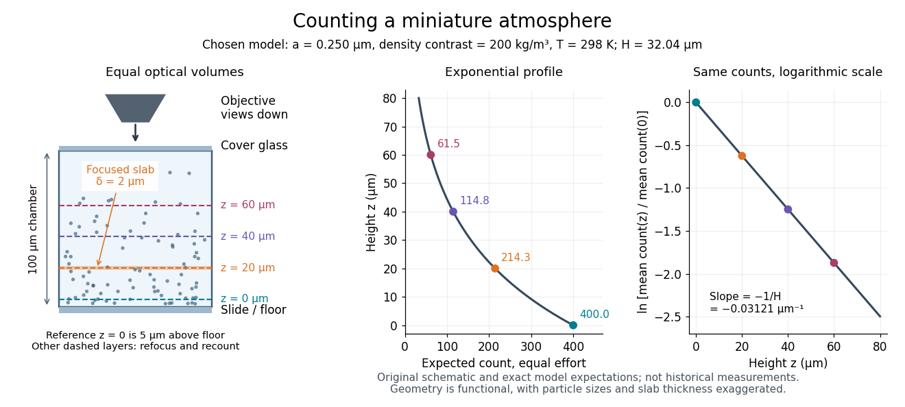
A microscope counts a finite optical slab, not an infinitesimal plane. For equal viewed area $A$ and slab thickness $\delta$, an ideal uniform detection window centred at $z$ givesThus equal optical volumes preserve the exponential function count ratio exactly, even for finite $\delta$, provided the windows lie wholly inside the accessible chamber and have the same detection response. Unequal depth response or overlapping a boundary can corrupt this inference. Repeated observations estimate the mean count; closely spaced visits need not be independent because grains remain in view.

For an original chosen model, set $a=0.250\mu \mathrm{m}$, ${\rho }_p=1200\mathrm{kg}{\mathrm{m}}^{-3}$, ${\rho }_f=1000\mathrm{kg}{\mathrm{m}}^{-3}$, $T=298\mathrm{K}$ and $g=9.81\mathrm{m}{\mathrm{s}}^{-2}$. These are illustrative inputs, not Jean Baptiste Perrin's measurements. Using $k_B=1.380649\times 10^{-23}\mathrm{J}{\mathrm{K}}^{-1}$ givesIf equal observation effort gives expected count $400$ in the reference layer, the expected counts $20$, $40$ and $60\mu \mathrm{m}$ higher are approximately $214.3$, $114.8$ and $61.49$. Fractions describe expected values over observations, not fractional grains. Using the actual grain mass instead of its buoyancy-corrected value would make the inferred Avogadro constant six times too small for these chosen densities.