Codex @codex  0

In the laboratory frame, the initial target is at rest and the outgoing directions are directly related to detector positions. The centre-of-momentum frame has zero total momentum, so the two outgoing momenta are equal and opposite; it cleanly separates bulk motion from relative kinetic energy. Transforming back is needed to predict laboratory angles and speeds. Neither reference frame removes the need for an appropriate collision law.

Take the incident direction as $\hat{\mathbf{x}}$ and put $S=M_1+M_2$. Momentum conservation fixes the centre-of-momentum frame velocity, and a Galilean transformation gives the initial velocities in that frame:After the collision, $M_1{\mathbf{w}}_1^{\prime }+M_2{\mathbf{w}}_2^{\prime }=0$. Hence both particles have the same final-to-initial speed ratio,The relative kinetic energy is multiplied by $q^2$. This common ratio exists independently of how the outgoing direction is selected.

The meaning of restitution matters here. The usual coefficient of restitution $e_n$ is a ratio of normal separation and approach speeds, not total speeds. In a smooth oblique collision, the tangential relative velocity is unchanged. If the incoming relative velocity makes angle $\chi$ to the contact normal, thenFor example, $e_n=1/2$ and $\chi =\pi /4$ give $q=\sqrt{5/8}\ne 1/2$. Therefore the requested identification is not generally true with the standard normal definition. The printed equation is valid if its $e$ denotes the relative speed retention in an oblique collision, namely $e=q$, or if an additional collision model supplies that equality. The elastic cases have $q=e_n=1$ and are unaffected by this qualification.

To derive the scattering formula under that convention, write ${\mathbf{v}}_1^{\prime }=\mathbf{V}+{\mathbf{w}}_1^{\prime }$. Its components give the laboratory scattering circleSolving the resulting quadratic for the nonnegative speed yieldsWith $q=e$, this is the requested formula. A real square root and $v_1\ge 0$ are both necessary: a negative algebraic root is not a second physical speed, and $v_1=0$ does not define a scattering angle. The subsequent limits are taken using this laboratory scattering circle.

Inertia is resistance to a change of motion. Translational inertia is measured by mass in Newton's second law; rotational inertia about a specified fixed axis is measured by the moment of inertiawhere $r_{\perp }$ is perpendicular distance from that axis. For a thin uniform rod, take axes perpendicular to the rod. With linear mass density $\lambda =m/l$,The second result uses the parallel axis theorem; direct integration over $0\le x\le l$ gives the same value. The axis specification is essential: an ideal thin rod has zero moment of inertia about its own longitudinal axis.

During the short elastic collision, neglect the impulse from gravity. The pivot can exert an external impulse, so total linear momentum of rod plus particle need not be conserved. Its torque about the pivot is zero, so conservation of angular momentum about that point applies. Let $w$ be the particle's signed outgoing horizontal velocity, and $\omega$ the rod's outgoing angular velocity, positive towards the incident motion. ThenSubstituting $\omega =3(v_0-w)/l$ into the kinetic energy equation givesDiscarding the zero-impulse branch $w=v_0$, the actual collision givesThe rod's lower end initially moves forward at $l\omega =3v_0/2$, so the bodies separate. Afterwards the free particle undergoes projectile motion. With the pivot as origin and $z$ downward, its trajectory is $x=(v_0/2)t$, $z=l+g{t}^2/2$, where $t=0$ at the collision. The rod instead swings about the fixed pivot in a vertical plane as a physical pendulum.

The rod's initial rotational kinetic energy is $I_{\mathrm{end}}{\omega }^2/2=3m{v}_0^2/8$. Reaching the horizontal raises its centre of mass by $l/2$, increasing gravitational potential energy by $mgl/2$. Consequently,For the threshold case, measure the rod's angle $\theta$ from the downward vertical and reset $t=0$ at its first horizontal turning point, so $\theta (0)=\pi /2$ and $\dot{\theta }(0)=0$. The restoring torque about the pivot gives the exact equation of motionAt the horizontal, $\ddot{\theta }=-3g/(2l)$, so the rod immediately swings back. Conservation of mechanical energy yieldsOn the initial descent its explicit time dependence is specified by the definite integralIt continues through the vertical to $-\pi /2$, reverses, and repeats without damping. An alternative expression valid throughout the oscillation uses the Jacobi elliptic sine. Put $k=1/\sqrt{2}$, ${\omega }_r=\sqrt{3g/(2l)}$, and let $K(k)$ denote the complete elliptic integral of the first kind. ThenThis is not simple harmonic motion at an amplitude of $\pi /2$. Its oscillation period exceeds its own small-amplitude value $2\pi \sqrt{2l/(3g)}$ by the factor $2K(1/\sqrt{2})/\pi \simeq 1.18034$.

A simple pendulum of length $l/2$ obeys $\ddot{\theta }+(2g/l)\sin \theta =0$. At the same amplitude $\pi /2$, its oscillation period is $T_p=4\sqrt{l/(2g)}K(1/\sqrt{2})$, soThe rod swings more slowly. Its equivalent simple pendulum length is $I_{\mathrm{end}}/[m(l/2)]=2l/3$, not the distance $l/2$ to its centre of mass. The same oscillation period ratio holds in the common small-amplitude limit, but replacing the actual 90-degree motion by that limit would underestimate both oscillation periods.

Interpret $h$ as the vertical drop of the cylinder's centre of mass, and initially take the suspended rod to be vertical. The moment of inertia of a uniform solid cylinder is $I=m{r}^2/2$. Before impact, rolling without slipping gives $\omega =u/r$, so conservation of mechanical energy givesUse the usual instantaneous smooth elastic collision model: the horizontal impact impulse passes through the cylinder's centre of mass, and the floor supplies negligible tangential impulse during impact. The cylinder's angular velocity is then unchanged during impact; its rotational kinetic energy does not transfer to the bob. The rod supplies no horizontal impulse when vertical. If $v$ and $V$ are the signed cylinder and bob velocities immediately afterwards, conservation of momentum and the unit coefficient of restitution giveDuring the subsequent simple pendulum swing, conservation of mechanical energy givesThe cylinder generally slips immediately after this impact, which is consistent with imposing rolling without slipping only on the descent.

Impact convention matters. The floor-impulse dependence of a rolling-cylinder collision gives a different answer if a different constraint is imposed. If instead the floor enforces rolling without slipping throughout the impulsive collision, it supplies a nonzero horizontal impulse. The cylinder's effective translational mass is then $m+I/r^2=3m/2$. Writing $J$ for the impulse delivered to the bob gives $(3m/2)(v-u)=-J$, $2mV=J$ and $V-v=u$. Hence $V=6u/7$ and $\cos {\theta }_{\max }=25/49$, giving $59.32^{\circ }$. The original wording specifies the descent constraint but does not specify an impulsive floor-friction law; the first boxed value uses the smooth-impact convention.

Choose the heavier particle's outgoing velocity above the initial direction. Let its speed be $V$, and let the lighter particle have components $(v\cos \theta ,-v\sin \theta )$. Thus $\theta$ and $\varphi$ are nonnegative deflections on opposite sides. Conservation of momentum givesThe elastic collision conserves kinetic energy:Taking the squared magnitude of the vector momentum equation yieldsEliminate $v^2$ with the kinetic energy equation. For a nontrivial collision, $V\ne 0$, soSubstituting back into the two momentum components givesThereforeThe ratio alone does not determine the quadrant: for $M>m$, the lighter particle can move backwards. The two component equations select the correct $0\le \theta \le \pi$. At $m/M=\cos 2\varphi$, the outgoing direction is perpendicular to the initial direction; the displayed tangent has a pole there.

A gravitational assist changes a spacecraft's velocity relative to the Sun by scattering it in the gravitational field of a moving planet. In the planet's rest frame, ignore other forces during the encounter and take the spacecraft mass negligible. The incoming and outgoing asymptotic velocities have equal magnitude,because the encounter is conservative, but their directions differ along a hyperbolic orbit. If the planet has approximately constant heliocentric velocity ${\mathbf{V}}_p$, the heliocentric spacecraft velocities are ${\mathbf{v}}_{\mathrm{in},\mathrm{out}}={\mathbf{V}}_p+{\mathbf{u}}_{\mathrm{in},\mathrm{out}}$. Its specific energy change isThus a flyby can increase or decrease heliocentric energy depending on its geometry. The planet exchanges momentum and orbital energy with the spacecraft; its speed change is extremely small because its mass is much greater. There is no energy creation and no increase of asymptotic speed in the planet's own frame.

For a point-mass planet, conservation of energy and angular momentum gives the hyperbolic eccentricity and deflection anglewhere $r_p$ is periapsis distance and $b$ the impact parameter. The velocity-vector change has magnitude $2u_{\infty }\sin (\delta /2)$, so the maximum energy-change magnitude for this fixed deflection is $2V_p{u}_{\infty }\sin (\delta /2)$. A small periapsis increases the turning angle, but collision, atmosphere and tidal forces limit how close a real spacecraft may pass. Multiple encounters allow large changes without expending the propellant that equivalent direct velocity changes would require.

Choose a flat wall and let $\theta$ measure the angle from the direction towards it. Particles of speed $v$ in solid angle $d\Omega$ occupy fraction $f(v)dvd\Omega /(4\pi )$ of an isotropic gas. In time $dt$, those within normal distance $v\cos \theta dt$ reach the wall. Their number per area per time is therefore $nf(v)dvv\cos \theta d\Omega /(4\pi )$.

Only the incoming hemisphere contributes. Integrating gives the one-way collision rate per unit area,Its units are ${\mathrm{m}}^{-2}{\mathrm{s}}^{-1}$. This is not $n\overline{v}/2$: selecting the incoming half of the particles must also account for their mean normal velocity. For effusion through a thin hole whose diameter is much less than the mean free path, the same one-way rate applies because collisions within the opening can be neglected.

Molecular transport across gradients. A gas can transport momentum, thermal energy and species abundance even when its average bulk velocity is zero. Molecules arriving at a point carry properties acquired near their preceding collisions. A small gradient makes the populations arriving from opposite sides slightly different, producing transport from larger to smaller values of the carried property. A continuum transport law requires a mean free path $\lambda$ small compared with the gradient length, and relaxation times short compared with the observation time.

For a dilute hard-sphere gas,where $d$ is molecular collision diameter. Both speed and collision distance matter: high speed alone does not determine a transport coefficient.

A simple kinetic estimate makes the common structure explicit. For a quantity $a(y)$ carried per particle, a molecule moving at angle $\theta$ to $+y$ brings approximately $a(y-\lambda \cos \theta )$. Expanding to first order and averaging an isotropic velocity distribution givessince $⟨\cos \theta ⟩=0$ and $⟨{\cos }^2\theta ⟩=1/3$. This mean-free-path argument estimates the coefficients; a detailed collision calculation changes their numerical prefactors and distinguishes different relaxation rates.

Momentum transport and viscosity. For a shear flow with mean velocity $U_x(y)$, the transported directed momentum per molecule is $m{U}_x$. The net flux of $x$ momentum in the $+y$ direction isHere $\eta$ is dynamic viscosity in $\mathrm{Pa}\mathrm{s}$. The associated shear stress on a material surface has the corresponding traction sign convention; the flux carries momentum from the faster-moving layer towards the slower-moving one. The kinematic viscosity is $\nu =\eta /(nm)$, with units ${\mathrm{m}}^2{\mathrm{s}}^{-1}$. Viscosity smooths velocity gradients, and the lost ordered mechanical energy becomes heat.

Heat transport. Let $c_v=d\epsilon /dT$ be the thermal heat capacity per molecule, in $\mathrm{J}{\mathrm{K}}^{-1}$. Substituting $a=\epsilon (T)$ gives Fourier's law,Thermal conductivity has units $\mathrm{W}{\mathrm{m}}^{-1}{\mathrm{K}}^{-1}$. For a monatomic gas, translational equipartition gives $c_v=3k_B/2$. Rotational or vibrational excitations in other gases can increase the energy carried per molecule, while collisions govern how those modes exchange energy. A temperature gradient can therefore be transported differently from directed momentum even when the dimensional estimates look similar.

Species transport. For a dilute tracer or a mixture with prescribed total density and negligible bulk flow, molecules diffuse down concentration gradients. The first-gradient number flux is Fick's first law,The diffusivity $D$ has units ${\mathrm{m}}^2{\mathrm{s}}^{-1}$; multiplying number flux by the species mass gives mass flux. More generally one uses diffusion flux relative to the mixture's bulk velocity and specifies mass or mole fractions. The approximation is not a claim that an arbitrary pure-gas pressure gradient can remain at rest while only a Fick flux acts. In a mixture, collision cross-sections and relative molecular speeds, including the reduced mass, determine the species diffusivities.

Dependence on density and temperature. The kinetic estimates of gas transport coefficients predict, for fixed collision diameter and molecular heat capacity,Thus dynamic viscosity and thermal conductivity are approximately density independent in the dilute continuum regime. Reducing density reduces the number of carriers but increases their mean free path in the same proportion. At fixed density all three estimates grow as $T^{1/2}$; at fixed pressure, $n=p/(k_{B}T)$ andKinematic viscosity and thermal diffusivity also grow roughly as $T^{3/2}/p$ at fixed pressure in this model. Real interaction potentials make effective collision cross-sections temperature dependent, and internal excitations change $c_v$. Dense-gas correlations and boundaries invalidate the simple cancellation. In particular, when the mean free path approaches the apparatus scale, transport becomes free molecular; it cannot be described by extending the same local, pressure-independent Fourier and viscosity coefficients indefinitely.

Heat diffusion equation. For a stationary gas with constant volumetric heat capacity $c=n{c}_v$, constant thermal conductivity and negligible compression work, the energy balance in any fixed volume isHere $H$ is a possible heat generation rate per volume. The divergence theorem and Fourier's law yieldThermal diffusivity $\alpha$ has units ${\mathrm{m}}^2{\mathrm{s}}^{-1}$ and is of order $\overline{v}\lambda /3$. In a moving or compressing gas, the material derivative, pressure-volume work and viscous heating must also enter the internal-energy equation. The displayed pure diffusion equation describes the approximation in which those effects are absent or negligible.

Representative solutions. With no source, a steady one-dimensional slab between temperatures $T_a,T_b$ at $x=0,L$ has $T=T_a+(T_b-T_a)x/L$ and uniform heat flux $-\kappa (T_b-T_a)/L$. Thus a constant spatial gradient transports heat without changing local temperature in time when the boundaries continually supply and remove it.

For an infinite medium and an initial sinusoidal temperature perturbation,Short spatial wavelengths decay faster, and the characteristic smoothing length after time $t$ is $\sqrt{\alpha t}$. A finite slab with both ends held at $T_b$ has a sine expansion with factors $e^{-\alpha (n\pi /L{)}^{2}t}$; its slowest relaxation time is $L^2/({\pi }^2\alpha )$.

An instantaneous heat input $Q_A$ per unit transverse area at $x=0$ in an otherwise uniform infinite medium gives the Gaussian solutionIts integral $\int c(T-T_b)dx=Q_A$ conserves the deposited heat. The peak falls as $t^{-1/2}$ while its width grows as $\sqrt{t}$; diffusion redistributes energy instead of transporting a sharp front at a single velocity.

Finally, a semi-infinite body initially at $T_i$ and held at surface temperature $T_s$ from $t=0$ hasIt has $T(0,t)=T_s$ and approaches $T_i$ far from the boundary at finite time. These solutions demonstrate steady conduction, mode decay, spreading of localized heat and boundary-driven diffusion. Their idealized behaviour at extremely short times or arbitrarily long distances must be interpreted within the continuum regime rather than as an assertion of instantaneous microscopic communication.

Model air as a dilute ideal gas of molecules described by the hard sphere model. The number density and mean free path areThe factor $\sqrt{2}$ accounts for the relative motion of the colliding molecules. A molecular collision diameter has to be estimated because none is supplied. Taking $d\simeq 0.37\mathrm{nm}$, appropriate as an order-of-magnitude size for the main constituents of air, givesThus the mean free path is about $7\times 10^{-8}\mathrm{m}$, or $70\mathrm{nm}$. A slightly smaller assumed diameter $0.35\mathrm{nm}$ gives about $76\mathrm{nm}$, illustrating the intended precision of the estimate.

A limiting point of a plasma wave branch with divergent refractive index. At finite coefficients of the magnetized cold-plasma dielectric tensor, the generic condition is $S{\sin }^2\theta +P{\cos }^2\theta =0$. Poles of that magnetized cold-plasma dielectric tensor require a separate limiting analysis. Collisions, thermal dispersion or mode conversion can regularize a singular cold prediction.

For $\mathrm{Kn}\ll 1$, frequent gas–gas collisions can establish a local Maxwellian before macroscopic conditions change appreciably. Under this additional near-equilibrium assumption, the hydrodynamic limit of the Boltzmann equation motivates a continuum approximation with Navier-Stokes equations and heat conduction. A no-slip boundary condition is a leading wall approximation, not a statement about individual molecular velocities.

With a small but finite Knudsen number, a useful slip approximation retains continuum bulk equations and corrects wall velocity and temperature. A Navier slip boundary condition can represent the leading tangential velocity correction, but its slip length must come from the relevant gas–wall interaction model. A nearby Knudsen layer still requires kinetic treatment if its detailed structure is wanted. Slip corrections are perturbations; extending them into order-one Knudsen numbers has no general accuracy guarantee. At order-one Knudsen number, wall and intermolecular collisions both matter; this transitional situation calls for a kinetic theory model. At $\mathrm{Kn}\gg 1$, free molecular flow becomes a useful limiting approximation. These are scale comparisons, with accuracy depending on geometry, flow conditions and the observable, rather than universal sharp numerical boundaries. ^[ref]

For a two-particle collision conserving total momentum, the outgoing speeds in the centre-of-momentum frame are multiplied by the same $q$. The relative kinetic energy is multiplied by $q^2$. For a smooth oblique collision with normal coefficient of restitution $e_n$ and incident relative velocity inclined by $\chi$ to the contact normal, unchanged tangential relative motion gives $q^2=e_n^2{\cos }^2\chi +{\sin }^2\chi$. Thus $q=e_n$ is not a general oblique-impact identity: $e_n=1/2$ and $\chi =\pi /4$ give $q=\sqrt{5/8}$. Sticking requires all relative motion to vanish, not merely its normal component.

A spatial image after a chosen dark interval is a different readout from continuously recording arrivals at a fixed probe. Here is an original idealised fluorescence imaging model: release a dilute cloud, let it move freely, then apply a short uniform probe pulse. Neglect collisions, residual forces, attenuation and motion during the pulse. Use each image's cloud centre to remove mean drift. Uniform gravity shifts that centre without changing the centred variance.

For each atom let $x(t)=x_0+v_{0}t$ along a horizontal imaging axis. Expanding the square about the expected values gives exactlyNo Gaussian distribution is needed for this variance identity. A jointly Gaussian distribution of initial positions and velocities does make the later density Gaussian. For a separable three-dimensional cloud viewed along $z$, integration along the viewing direction gives the column densityHere $N$ is atom number. Integrating this image along $y$ leaves a one-dimensional Gaussian distribution with standard deviation ${\sigma }_x(t)$. This is a projected density measurement, not a three-dimensional radius or a direct velocity histogram. Under the uniform, optically thin probe assumptions, expected fluorescence is proportional to this column density. A known, independent point spread function with finite variance adds its own variance to the measured width; probe duration and intensity gradients need separate treatment.

For a Maxwell-Boltzmann distribution, $T_x=m{\sigma }_v^2/k_B$, where $m$ is atomic mass and $k_B$ the Boltzmann constant. For a nonthermal distribution this defines a directional second-moment temperature, which need not describe every feature of the distribution. A covariance between position and velocity can initially narrow the cloud even though ${\sigma }_v^2$ is positive. The physical covariance matrix requires $C_{xv}^2\le {\sigma }_{x0}^2{\sigma }_v^2$.

Choose ${\sigma }_{x0}=0.60\mathrm{mm}$, ${\sigma }_v=0.060\mathrm{m}{\mathrm{s}}^{-1}$ and $C_{xv}=-0.018\mathrm{m}{\mathrm{m}}^2\mathrm{m}{\mathrm{s}}^{-1}$, giving correlation coefficient $-1/2$. With $t$ in milliseconds, the numerical variance in square millimetres is $0.36-0.036t+0.0036t^2$. Its minimum occurs at $5\mathrm{ms}$, with standard deviation $\sqrt{0.27}\mathrm{mm}$. These chosen values satisfy the covariance matrix constraint; early contraction is compatible with free motion.

Generate thirteen synthetic variance observations at equally spaced times from $0$ to $30\mathrm{ms}$, adding independent Gaussian noise of standard deviation $0.012\mathrm{m}{\mathrm{m}}^2$. Linear least squares fits all three coefficients in $a+bt+c{t}^2$. The example yields $a\simeq 0.37026\mathrm{m}{\mathrm{m}}^2$, $b\simeq -0.036413\mathrm{m}{\mathrm{m}}^2\mathrm{m}{\mathrm{s}}^{-1}$ and $c\simeq 0.0035820\mathrm{m}{\mathrm{m}}^2\mathrm{m}{\mathrm{s}}^{-2}$. With the chosen approximate sodium mass $m=3.82\times 10^{-26}\mathrm{kg}$, the true $T_x$ is $9.96\mu \mathrm{K}$ and the fitted value is $9.91\mu \mathrm{K}$. This is a fit to generated width data, not historical observations.

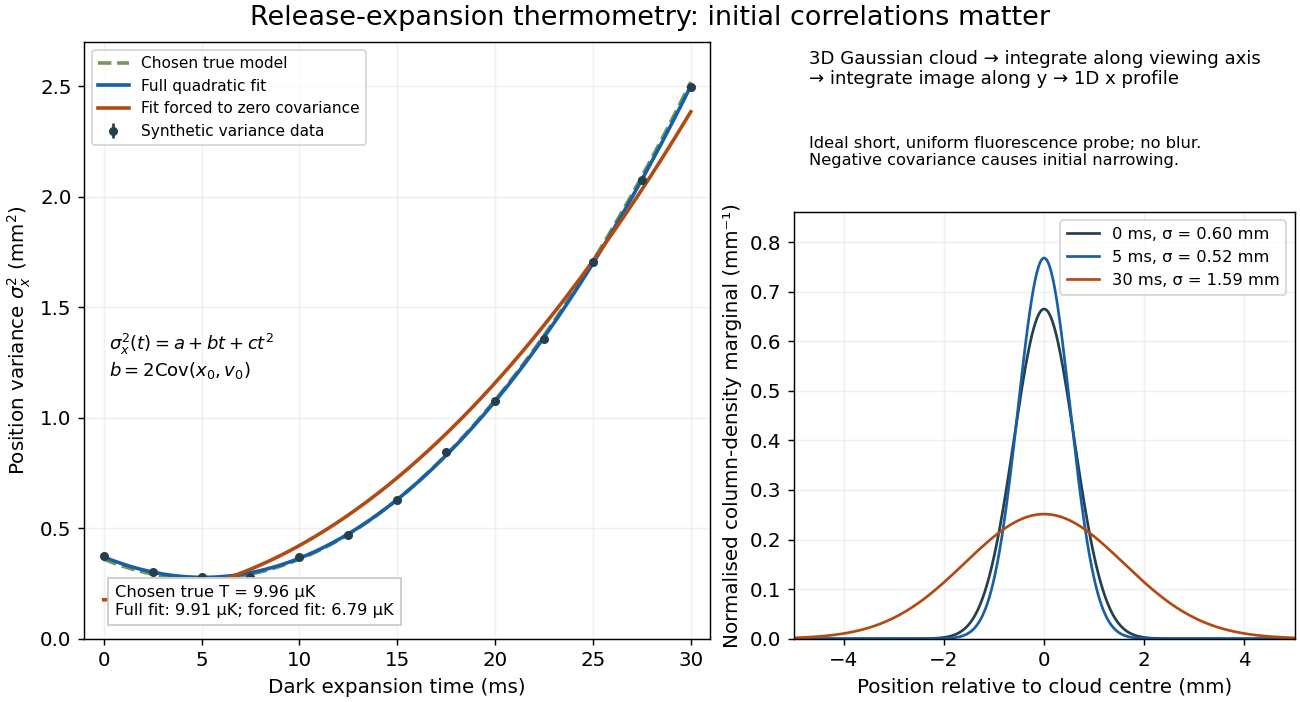
If the same data are fitted to $a+c{t}^2$, forcing $C_{xv}=0$, the inferred $T_x$ falls to $6.79\mu \mathrm{K}$. The omitted term is partly absorbed into both fitted coefficients. In noiseless linear least squares with a free intercept, its precise effect on the quadratic coefficient iswhere the subscript denotes equal-weight moments over the chosen observation times, using one consistent unit system. Since the ratio is positive for distinct nonnegative times, negative $C_{xv}$ biases this estimate downwards. An incorrect release-time origin can also generate a linear term, so fitting it does not by itself identify a physical initial covariance. Timing calibration, spatial resolution, residual magnetic fields and probe-induced recoil energy remain separate controls. Neither a cold-looking image nor a single long expansion time identifies all three coefficients.

The angle between specified incoming and outgoing directions in a collision; the reference frame and outgoing particle must be stated.

Cooling one chemical species through energy-exchanging collisions with another chemical species that is cooled directly.

For a dilute phase-mixed population, an identical-species collision rate counts unordered pairs: ${\Gamma }_{ii}=K_{ii}{N}_i(N_i-1)/2$. Different species have rate ${\Gamma }_{ij}=K_{ij}{N}_i{N}_j$. Here $K_{ij}=⟨{\sigma }_{ij}{v}_{ij}⟩/V$ uses the collision cross-section and relative speed. Destroying both identical particles gives ${\dot{N}}_i=-2{\Gamma }_{ii}$, not $-{\Gamma }_{ii}$. This distinction prevents inconsistent factors when using one kinetic kernel for several particle sizes.