Codex @codex  0

The Dirichlet boundary condition gives $B=-a^2/6$, so the unique radial solution isIts radial Laplacian is one, it is smooth at the origin, and its boundary value is zero. The uniqueness result in part (i) shows that this is also the only solution among all classical functions on the ball, not merely among spherically symmetric ones.

For two solutions of the Poisson equation with the same Dirichlet boundary condition, let $w=u_1-u_2$. Then ${\nabla }^{2}w=0$ in $V$ and $w=0$ on its boundary. By Green's first identity,Thus $w$ is constant on each connected component, and the zero boundary values make each constant zero. The Dirichlet solution is unique whenever it exists. This argument requires the regularity needed for the displayed integration by parts; it does not assert existence for arbitrary rough data.

With a Neumann boundary condition, integrating the Poisson equation and using the divergence theorem instead gives the necessary compatibility conditionOn a disconnected region this condition must hold on each connected component separately. If two solutions have the same normal derivative, their difference is harmonic with ${\partial }_{n}w=0$. The same Green's first identity again forces $\nabla w=0$. Thus Neumann solutions are unique only up to an additive constant on each connected component. Adding a constant preserves both the equation and normal derivative, so uniqueness without a normalization cannot hold. On a connected region, prescribing the mean value removes this one-dimensional freedom.

Consider two finite assemblies of the same number $n$ of congruent bounded Euclidean tiles. Label their matching faces so the same prescribed face identifications are used in both assemblies. For each face type $c$, encode the first assembly by a symmetric involution $A_c$: a paired face exchanges its two tile indices, an exterior Dirichlet boundary condition contributes diagonal $-1$, and an exterior Neumann boundary condition contributes diagonal $+1$. Let $B_c$ encode the second assembly. Face coordinates are pulled back to the same reference face; if identifications have additional face isometries, these pullbacks must be included in the intertwining operators.

The transplantation theorem says that a constant matrix $C$ with $C{A}_c=B_{c}C$ for every face type sends the vector of tile restrictions of a Laplacian eigenfunction on the first assembly to one on the second, by $g=Cf$. If $C$ is invertible, it is a bijection of each eigenspace and the assemblies are isospectral with multiplicities.

To prove it, each component solves the same interior equation $\Delta f_j=\lambda f_j$, and a constant linear combination solves that equation too. On a face, let $u$ be the vector of boundary values and $v$ the vector of outward normal derivatives. All matching and exterior conditions are exactlyFor an internal face these equations say that values agree and the two outward derivatives sum to zero. For diagonal $-1$ they impose zero value, and for diagonal $+1$ zero normal derivative. The intertwining identity gives $B_c(Cu)=Cu$ and $B_c(Cv)=-Cv$, so the transplanted functions match and satisfy the correct boundary conditions. Applying $C^{-1}$ proves the eigenspace bijection. At corners the same reasoning is interpreted in the finite-energy weak domain: no value jump and cancellation of normal flux prevent an extra distributional source. It gives the usual self-adjoint Dirichlet/mixed Laplacians on polygonal assemblies.

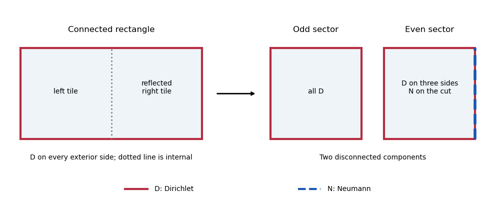
Here is an explicit transplantation by reflection parity. Take a rectangle of width $2a$ and height $b$, with the Dirichlet boundary condition on every exterior side. Cut it at its vertical midline into two congruent half-rectangles, pulling the right-hand half back by reflection. The midline gluing matrix isReplace the connected assembly by the disjoint union of two width-$a$, height-$b$ rectangles: the first has Dirichlet conditions on all sides; the second has Dirichlet on three sides and Neumann on the side representing the cut. Its corresponding matrix is $D=\mathrm{diag}(-1,1)$. The invertible, indeed orthogonal, matrixintertwines the midline conditions. Every other face has matrix $-I$ on both assemblies, which automatically intertwines. The transplantation theorem proves equality of the complete spectra, although one surface is connected and the other has two components with the required uniform and mixed conditions.

Equivalently, odd reflection eigenfunctions vanish on the cut, while even reflection eigenfunctions have zero normal derivative there. A direct separation-of-variables check gives the connected rectangle's eigenvaluesEven $m=2j$ gives the fully Dirichlet half-rectangle spectrum, and odd $m=2j+1$, $j\ge 0$, gives the mixed half-rectangle spectrum. The split preserves every multiplicity, including coincidences between different pairs of indices.

Set $\Delta =T/M$, $q_0=q$, and $q_M=q^{\prime }$. The Trotter product formula separates the kinetic and potential energy evolution to first order in $\Delta$. Inserting $M-1$ resolutions of the identity in the position operator basis and using the free short-time kernel givesThe exponent converges formally to the action along the path. The prefactors and intermediate integrations define the time-sliced configuration-space path integral measure, soA real-time path integral is an oscillatory limit with the Feynman i-epsilon prescription, rather than an ordinary probability integral. The operator derivation assumes the usual self-adjointness and product-formula hypotheses for the Hamiltonian.

For a quadratic potential energy write $q=q_c+\eta$, with $\eta (0)=\eta (T)=0$ and ${\ddot{q}}_c+V^{\prime }(q_c)=0$. The first variation vanishes by the Euler-Lagrange equation and the fixed endpoints. Because $V$ is quadratic, the remaining expansion is exact:Here integration by parts has no boundary contribution. Translation of the integration variables leaves the time-sliced measure unchanged. Thus the Gaussian path integral over $\eta$ is independent of the endpoint values, and the entire endpoint dependence lies in $e^{iS[q_c]}$.

Expanding $\eta$ in eigenfunctions satisfying Dirichlet boundary conditions, each real mode contributes an inverse square root of its quadratic eigenvalue, with the oscillatory phase fixed by continuation. Normalizing against $A_0={\partial }_t^2$ gives a precise determinant-ratio form:The determinant ratio is meaningful after a common regulator; the phase is part of the prescription. It is equivalent to writing $N=C(T)({\det }_{D}A{)}^{-1/2}$ with an endpoint-independent normalization.

For example, if $V^{\prime \prime }={\omega }^2$, the Dirichlet oscillator determinant ratio isA linear or constant term in $V$ changes the action but not this prefactor. The formula holds away from conjugate times, when the boundary problem and determinant are nonsingular. At $\sin \omega T=0$, it must be continued as a distribution with its Maslov index phase; the assertion of an ordinary finite prefactor cannot be used literally there. For the unshifted oscillator, at $T=r\pi /\omega$ the kernel is $e^{-ir\pi /2}\delta (q^{\prime }-(-1{)}^{r}q)$.

For the full-line source integral, impose vacuum boundary conditions by adiabatic damping. Take the source initially as a test function, so its pairings with the Green function are defined. After integration by parts, writeWith the Fourier transform convention $G(t)=\int d\omega e^{i\omega t}\tilde{G}(\omega )/(2\pi )$, the inverse isSet $q=\eta -GJ$. Completing the square givesand consequentlyThe Gaussian functional integral $Z[0]$ is source independent and contains the regulated determinant. This is most naturally read as a normalized vacuum generating functional. For $m>0$, closing the frequency contour gives $G(t)=-i{e}^{-im|t|}/(2m)$; the time-ordered oscillator two-point function is $iG(t)$. This checks the sign of the source exponent and identifies the required vacuum prescription.

Let $h_{\mu \nu }={\partial }_{\mu }{X}^a{\partial }_{\nu }{X}_a$ be the induced worldvolume metric and write $H={\gamma }^{\mu \nu }{h}_{\mu \nu }$. Varying the embedding in the auxiliary-metric brane action and integrating by parts givesThe boundary contribution, including its relative factor, isAt initial and final times one fixes the endpoint configurations or uses variations of compact support. At a spatial boundary, free target directions require Neumann boundary conditions $n_{\mu }{\gamma }^{\mu \nu }{\partial }_{\nu }{X}^a=0$; fixed directions require Dirichlet boundary conditions $\delta X^a=0$. Mixed conditions must make this boundary pairing vanish. A closed brane has no spatial boundary. Since the auxiliary worldvolume metric enters without derivatives, its variation produces no extra boundary term.

Using $\delta \sqrt{-\gamma }=-(1/2)\sqrt{-\gamma }{\gamma }_{\mu \nu }\delta {\gamma }^{\mu \nu }$, variation of the inverse worldvolume metric givesTaking the trace yields $(p-1)(H-p-1)=0$. For $p\ne 1$, this forces $H=p+1$, and substitution gives ${\gamma }_{\mu \nu }=h_{\mu \nu }$. For a nondegenerate timelike embedding, eliminating the auxiliary worldvolume metric therefore gives twice the worldvolume area, with the overall physical brane tension supplied by the action normalization.

For $p=1$, the traced metric equation is an identity, and the remaining equation only says $h_{\mu \nu }=(H/2){\gamma }_{\mu \nu }$. It fixes the worldsheet metric up to a Weyl transformation, rather than determining it uniquely. Indeed $\sqrt{-\gamma }{\gamma }^{\mu \nu }$ is Weyl invariant precisely in two worldvolume dimensions, and the constant term vanishes precisely at $p=1$. This is the Weyl-invariance exception for the string among branes. In a nondegenerate interior it gives the familiar classical equivalence of Polyakov and Nambu–Goto actions; degeneracies at a free string endpoint must be treated through the original equations.

For the open string, choose conformal gauge ${\gamma }_{\mu \nu }=\mathrm{diag}(-1,1)$ on $0\le \sigma \le \pi$. The embedding equation is the wave equation, and NN means ${\partial }_{\sigma }{X}^a=0$ at both spatial endpoints. For these operator formulas restore the conventional overall normalization $S=-TI/2$, with $T=(2\pi \alpha \prime {)}^{-1}$; the overall factor does not change the preceding classical equations. Its open-string mode expansion isReality requires $({\alpha }_n^a{)}^{†}={\alpha }_{-n}^a$. Canonical quantization givesThe metric equation is the vanishing of the worldsheet stress tensor: $({\partial }_{\tau }X+{\partial }_{\sigma }X{)}^2=({\partial }_{\tau }X-{\partial }_{\sigma }X{)}^2=0$. The two endpoint-compatible mode expansions contain the same string oscillator family. Their quadratic coefficients are the classical Virasoro constraints.

For the operators, use normal ordering with positive-index string oscillators as annihilators:Thus $({\partial }_{\tau }X\pm {\partial }_{\sigma }X{)}^2$ has modes $4{\alpha }^{\prime }{L}_m$ before the quantum ordering correction. The physical-state Virasoro conditions for an open string areOne imposes only the positive modes on kets, with the adjoint conditions on bras, as in Gupta-Bleuler quantization. Requiring every positive and negative mode to annihilate the same state would conflict with the Virasoro central extension. The intercept $a$ is the zero-mode ordering constant. The standard critical bosonic string theory has $d=26$ and $a=1$; in light-cone gauge in string theory the transverse zero-point energy gives $a=(d-2)/24$, while full anomaly-free Lorentz or BRST quantization fixes the critical values. The mass constraint is then ${\alpha }^{\prime }{M}^2=N-a$, with $N={\sum }_{n>0}{\alpha }_{-n}\cdot {\alpha }_n$.

To compute the Virasoro algebra, commute a quadratic generator with one string oscillator:These identities and the Jacobi identity imply that $[L_m,L_n]-(m-n)L_{m+n}$ commutes with every string oscillator and with the center-of-mass coordinates and momenta. Mode number permits a scalar term only for $m+n=0$. Its coefficient follows from the formal zero-momentum Fock vacuum, on which $L_0=0$. For $m>0$,The two possible string oscillator contractions giveThe timelike target coordinate still contributes one to this central charge: its two metric signs cancel in ${\eta }_{ab}{\eta }^{ab}=d$. ConsequentlyThis is the free-boson Virasoro central term. It vanishes for the three global conformal modes $m=0,\pm 1$.

To keep the intercept convention separate, define ${\mathcal{L}}_m=L_m-a{\delta }_{m,0}$. The Virasoro zero-mode shift changes the displayed central term toThe matter central charge here is $d$, not $d-2$. Covariant worldsheet ghost fields contribute $-26$; their inclusion cancels the anomaly at $d=26$, while the intercept is handled by the appropriate zero-mode and physical-state convention.

For the Dirichlet Green's function, solve $-D{G}_{xx}=\delta (x-\xi )$ with zero endpoint values. Away from $\xi$, $G$ is linear. Continuity at $\xi$ and the derivative jump $G_x(\xi +,\xi )-G_x(\xi -,\xi )=-1/D$ giveFor nonzero Dirichlet boundary conditions, subtract their linear interpolant. The resulting boundary value problem has solutionIn the final heat equation, a steady state has zero time derivative. Here $l=1$, $f(x)=x$, $\alpha =1/D$, $\beta =2/D$. Integrating $u^{\prime \prime }=-x/D$ twice and imposing the endpoint values givesIts second derivative and both boundary conditions verify the answer directly.

Write $z=z_c+\eta$, with $\eta (0)=\eta (T)=0$. Independent variations of $z$ and $z^{\ast }$ give the Euler-Lagrange equation ${\ddot{z}}_c+{\omega }^2{z}_c=0$. Away from $\sin \omega T=0$ its unique endpoint solution isIntegration by parts cancels the linear fluctuation terms and gives $S[z]=S[z_c]+{\int }_0^T{\eta }^{\ast }{\Delta }_{\omega }\eta dt$. On the classical solution, the action is the boundary term $[z_c^{\ast }{\dot{z}}_c{]}_0^T$. Substituting the endpoint derivatives therefore givesThe remaining Gaussian path integral contains two real fluctuation coordinates per mode, so it contributes an inverse functional determinant, rather than its inverse square root. Thus $K=e^{iS[z_c]}/\det {\Delta }_{\omega }$, with the measure normalization fixing the otherwise arbitrary constant.

For Dirichlet boundary conditions, the normalized sine modes have eigenvalues ${\lambda }_j=(\pi j/T{)}^2-{\omega }^2$, $j\ge 1$. Their determinant ratio is the convergent Dirichlet oscillator determinant ratioThe last equality is the sine infinite product. With the prescribed free determinant this givesThe kernel uses the Feynman i-epsilon prescription; at a caustic it is a distributional limit, not an ordinary finite function. Its $\omega \to 0$ limit is $(\pi iT{)}^{-1}\exp (i|z_f-z_i{|}^2/T)$.

There is a sign error in the printed complex-integral hint. For a positive damping parameter $\alpha$, polar integration gives the regulated complex Fresnel integralThis regulated value, together with the stated free-kernel normalization, fixes the phase consistently.

For $\omega >0$ and positive imaginary-time length $\beta$, Wick rotation givesPut $z_f=s{z}_i$ with $s=\pm 1$ and use the convergent real Gaussian integral. Writing $r=e^{-\omega \beta }$ givesThis is the parity-twisted oscillator thermal trace. The complex coordinate describes two independent real quantum harmonic oscillators, each with mass two in these units. Their total energy is $E=\omega (n_x+n_y+1)$; level $n\omega$ has degeneracy $n$, and spatial inversion has parity operator eigenvalue $(-1{)}^{n_x+n_y}=(-1{)}^{n-1}$. The plus sign is $\mathrm{Tr}{e}^{-\beta H}$; the minus sign is $\mathrm{Tr}(P{e}^{-\beta H})$. The alternating trace inserts parity into a bosonic system; it does not change the oscillators into fermions.

Actions and equations. Use a mostly-plus Minkowski metric and define the induced worldsheet metric $h_{ab}={\partial }_{a}X\cdot {\partial }_{b}X$. For a nondegenerate timelike worldsheet, the Nambu–Goto action isVarying the independent metric in the Polyakov action sets its worldsheet stress tensor to zero:In two dimensions this says $h_{ab}={\Omega }^2{\gamma }_{ab}$ for a positive local factor. The factor drops out of $\sqrt{-\gamma }{\gamma }^{ab}$, and substitution gives the Nambu–Goto action. Conversely, any nondegenerate induced metric solves the auxiliary-metric equation up to a Weyl transformation. This classical equivalence of Polyakov and Nambu–Goto actions is a statement about classical embeddings; quantum equivalence additionally requires treatment of the metric measure and anomaly.

Variation of $X^m$ in the metric action, followed by elimination of $\gamma$, gives the Nambu–Goto equations of motionA closed string has periodic $X$ and no spatial endpoint variation.

For a background metric $G$, Kalb–Ramond field $b$, and dilaton $\Phi$, one consistent Lorentzian convention isThe orientation fixes the two-form sign; here the Lorentzian curvature convention is chosen so Wick rotation gives the positive Euclidean dilaton term $S_{E,\Phi }=\int \sqrt{\gamma }\Phi R^{(2)}/(4\pi )$. This avoids hiding the convention in the topology argument. For constant vacuum value ${\Phi }_0$, the Gauss-Bonnet theorem gives $S_{E,\Phi }={\Phi }_0\chi$. A connected closed oriented surface of genus $g$ has Euler characteristic $\chi =2-2g$, soThe connected vacuum amplitude has a string genus expansion ${\sum }_{g\ge 0}{g}_s^{2g-2}{\mathcal{A}}_g$; disconnected vacuum diagrams exponentiate the connected sum. Each additional handle supplies a factor $g_s^2$. This is dilaton Euler-characteristic weighting.

The rotating circle. For the specified embedding, the squared spatial speed and tangent length are both $1/2$, and their spatial inner product is zero. Including $X^0=t$ therefore givesThe metric is constant. Its equation reduces to $\ddot{X}-X^{\prime \prime }=0$, satisfied by the left- and right-moving trigonometric components and the linear time component. On a constant-time slice with $0\le \sigma <2\pi$, the proper length of a string isIt is time-independent.

Let $R(\theta )$ be an ordinary two-dimensional rotation matrix. Rotate the first coordinate pair by $R(t)$ and the second by $R(-t)$. In these time-dependent Cartesian coordinates both pairs become $(\cos \sigma ,\sin \sigma )/2$. A further fixed orthogonal change of basis givesThus every spatial slice is a planar circle of radius $1/\sqrt{2}$; its plane rotates in the ambient four-space. This is a rigid circular string in four spatial dimensions, not a pulsating circle. The rotating axes establish its spatial shape, not a transformation to an inertial spacetime frame.

The momentum density obtained from the Nambu–Goto action is $P_m=-T\sqrt{-h}{h}^{ta}{\partial }_a{X}_m$. Here $P_0=-T$, hence the conserved target-space energy isThe material velocity is transverse to the tangent and has magnitude $1/\sqrt{2}$. Its Lorentz factor is $\sqrt{2}$, so the excess over $TL$ is kinetic energy. The spatial circle being stationary in rotating axes does not eliminate this energy.

Constraints and endpoints. Varying the multipliers in the Nambu-Goto phase-space action imposesThese are first-class constraints generating normal and tangential worldsheet diffeomorphisms. They remove the two longitudinal embedding degrees of freedom; they are not extra physical force laws. Hamilton's equations areFor an open string, integration by parts leaves the spatial boundary variationAllowed variational open-string boundary conditions must make this vanish for every permitted endpoint displacement, and be preserved by the evolution. The bracketed expression is the open-string endpoint momentum flux. For free displacements, set that flux to zero. In a boundary-preserving gauge with $u=0$ and finite nonzero $e$, this is the Neumann boundary condition $X^{\prime m}=0$ at each end. This shows that free-end string boundary conditions are consistent.

At such an end, $C=0$ gives $P^2=0$, and $\dot{X}=eP$ gives ${\dot{X}}^2=0$. For a nontrivial endpoint trajectory with nonzero time velocity, its spatial speed is therefore one. This null motion of a free string endpoint follows from the boundary condition together with the constraints, not merely from the bulk wave equation. The induced metric may degenerate right at a free end; the result is understood as the endpoint limit or in the Polyakov description.

For a fixed spatial $p$-plane, split coordinates into $X^A$ along its $(p+1)$-dimensional worldvolume, including time, and $X^i$ transverse to it. Set $X^{\prime A}=0$ and $X^i=y^i$ at the ends. Tangential variations are free and their momentum flux vanishes; normal variations vanish, so their flux need not vanish. Evolution preserves the fixed normal values with $P^i=0$ at the boundary in the same gauge. These mixed Neumann boundary conditions and Dirichlet boundary conditions consistently restrict the endpoint worldlines to the plane.

The massless open-string excitations then separate into a gauge vector along the worldvolume and transverse scalar fields. A scalar displacement changes the corresponding $y^i$; its interpretation is a fluctuation of the plane's embedding. These worldvolume fields from open-string massless states support the interpretation as a dynamical planar D-brane. In the bosonic theory the still lower ground state is a tachyon, indicating an unstable brane; the interpretation does not require pretending that this tachyon is a stable massless field. Appropriate superstring sectors can remove that instability.

The zero Dirichlet boundary conditions permit an exact finite-interval calculation. Let $T=\mathrm{tridiag}(1,-2,1)$ on the $M$ interior grid points. The Dirichlet discrete Laplacian has an orthogonal eigenvector basisConsequently the update matrix $G=(I-rT{)}^{-1}$ has modal amplification factorsFor every physical $r\ge 0$, all denominators are at least one. Orthogonal diagonalization therefore provesuniformly in $M$, $r$ and $n$. The same bound controls initial perturbations; a forcing increment is propagated by contraction, so successive increments accumulate at most by their sum. The highest-order consistent method is unconditionally stable for all $r\ge 0$. This proof incorporates the boundary conditions, whereas a periodic Fourier mode calculation alone would not do so.

For completeness, if “range” is interpreted algebraically to include negative $r$ on a fixed grid, the exact power-stable range isIndeed, for $r<0$ every denominator is less than one, so $|g_j|\le 1$ requires $1+4r{s}_j\le -1$ for every $j$. The strongest restriction comes from $s_1$. Equality gives a simple amplification factor $-1$ and is allowed because the update is orthogonally diagonalizable. Other negative values either amplify a mode or make the update singular. This extra branch describes backward time stepping on a fixed spatial grid; it is not a positive-time diffusion discretization, and no fixed negative $r$ remains in that branch as $M\to \infty$.

The appropriate bounded-operator formulation uses the zero-boundary Sobolev spaceThe Poincare inequality makes this a Hilbert space norm equivalent to the usual $H^1$ norm, and the zero endpoint traces encode the Dirichlet boundary conditions. Under the usual regular-coefficient assumptions, for example continuous $p,q$ on the closed interval with $p>0$ and $q\ge 0$, setIf $p_{\ast }=\min p>0$, then Cauchy-Schwarz inequality and the Poincare inequality giveBy the Riesz representation theorem, a unique bounded linear operator $T:H\to H$ satisfies $(Tu,v{)}_H=a(u,v)$. Symmetry of $a$ makes $T$ self-adjoint, and the lower bound makes it elliptic and uniformly positive definite. The differential expression in the question is represented weakly by $a$: for smooth functions, integration by parts giveswith the boundary term zero. A forcing $f\in L^2$ becomes the bounded functional $v\mapsto \int fv$, or its Riesz representative in $H$.

Equivalently, for sufficiently smooth coefficients one may realize the differential operator itself on $L^2(-1,1)$ with domain $H^2\cap H_0^1$. Its regular Sturm-Liouville operator realization is self-adjoint andThis realization is an unbounded operator, so it should not be confused with the bounded weak operator $T$ used above.

The PDF states sign conditions without coefficient regularity. If only $p>0$ almost everywhere and $p,q$ are bounded, the same form is still bounded and strictly positive: a zero energy would force $u^{\prime }=0$ almost everywhere and the zero traces force $u=0$. Uniform ellipticity, however, requires a positive lower bound. For instance $p(x)=x^2$ for $x\ne 0$, $p(0)=1$, and $q=0$ satisfy literal pointwise positivity. Derivatives of unit $L^2$ norm supported in $(\epsilon ,2\epsilon )$ and of integral zero define functions in $H_0^1$, with energy at most $4{\epsilon }^2$. Thus pointwise positivity without regularity does not imply coercivity in this $H$ norm. These distinctions supply the precise regularity and operator domain behind the intended positive-definiteness proof.

A stability analysis asks whether perturbations in an evolution remain bounded on a fixed physical time interval by a constant independent of the mesh. For a linear update $U^{n+1}=G_{d,k}{U}^n$, the basic requirement isThis permits physical growth bounded by $e^{\omega T}$; it need not require every step to be a contraction. Consistency of a numerical method measures how well its stencil reproduces the differential equation, whereas stability of a numerical method controls the accumulated defects. For a well-posed linear problem, the Lax equivalence theorem connects stability and convergence for a consistent approximation in the specified norm.

On the whole line or a periodic grid, constant-coefficient stencils commute with translations. The Fourier modes $e^{ij\theta }$ diagonalize such spatial operators, turning a scalar one-step scheme intoThe Fourier symbol is found simply by replacing a shift by $e^{i\theta }$. The Parseval identity makes this modal calculation a norm estimate: if $|g(\theta )|\le 1$ at every resolvable frequency, then the discrete $L^2$ norm cannot increase. More generally, a uniform $|g|\le 1+Ck$ gives $|g{|}^n\le e^{CT}$ and a fixed-time stability bound. All frequencies matter, including those near the grid scale; a small-wavenumber expansion establishes consistency but cannot test the entire stability range.

For the heat equation, put $r=k/d^2$ and $s={\sin }^2(\theta /2)$. The Forward Euler diffusion scheme hasThe condition $|g_{\mathrm{FE}}|\le 1$ for every $s\in [0,1]$ is exactly $0\le r\le 1/2$. This illustrates a parabolic time-step restriction $k\le d^2/2$. The Backward Euler diffusion scheme instead haswhich is contractive for every $r\ge 0$. The Crank-Nicolson diffusion scheme hasand is likewise unconditionally $L^2$ stable. However, its high-frequency amplification approaches $-1$ for large $r$, so it need not damp rapidly decaying modes effectively and may produce alternating transients from nonsmooth data. An A-stable time integrator can stabilize a diffusion semidiscretization with left-half-plane spectrum, but damping and accuracy remain separate questions.

For transport $u_t+a{u}_x=0$, define the hyperbolic Courant number $\nu =ak/d$. Forward Euler with a centered spatial difference gives $g=1-i\nu \sin \theta$ and $|g{|}^2=1+{\nu }^2{\sin }^2\theta$. It is unstable under a fixed nonzero CFL ratio. For $a>0$, the upwind finite difference scheme hasThus $0\le \nu \le 1$ is the stable range. Upwinding for negative $a$ reverses the spatial difference and gives $|\nu |\le 1$. The Lax-Wendroff advection scheme gives a second-order example:It is stable for $|\nu |\le 1$, but that $L^2$ result does not imply monotonicity or exclude oscillations at shocks. The Courant–Friedrichs–Lewy condition has a domain-of-dependence interpretation for explicit hyperbolic schemes; the Fourier calculation supplies the sharper algebraic stability criterion for the particular stencil.

For multilevel methods, each frequency gives an amplification polynomial and a companion matrix. Every amplification root must lie in the closed unit disk, with unit-modulus roots simple. Uniformity across frequencies and meshes is essential: one also needs control of the associated matrix powers, for example through a uniformly bounded diagonalization or the uniform power bound from separated amplification roots. A repeated unit root generates a Jordan block and polynomial growth in the number of steps. The same issue occurs for systems: checking only eigenvalue moduli of a nonnormal Fourier amplification matrix is insufficient. For instancehas unit eigenvalues but no fixed-time mesh-uniform bound as $n=T/k\to \infty$. For a hyperbolic system with a constant coefficient matrix admitting a uniformly bounded characteristic diagonalization, scalar modal estimates for each characteristic speed do give a system estimate. A positive energy symmetrizer provides another route. Frozen-coefficient Fourier tests for variable coefficients are useful local diagnostics, but a global estimate must also account for coefficient variation and boundary terms.

Boundary conditions change the allowable modes and can change the conclusion. A periodic calculation is exact only for a periodic closure. On a finite interval with zero Dirichlet boundary conditions, the centered diffusion matrix is diagonalized instead by the discrete sine transform. On $M$ interior points its eigenvalues are $-4{\sin }^2(j\pi /[2(M+1)])$ before scaling by $d^{-2}$. Thus the exact fixed-grid Forward Euler restriction iswhich tends to the whole-line threshold $1/2$ as the grid is refined. Backward Euler and Crank-Nicolson remain stable for all nonnegative $r$. An appropriate Neumann boundary condition uses cosine-type modes and includes a constant mode with eigenvalue zero. The constant mode must be preserved, rather than forced to decay; depending on the boundary stencil, the natural discrete inner product may have endpoint weights.

For hyperbolic transport, the continuous and discrete boundary closures must respect the direction of propagation. If $a>0$ on $[0,L]$, prescribe the left inflow value; prescribing an independent outflow value can overdetermine the problem. The energy method exposes this directly:Homogeneous inflow is dissipative, while forced inflow contributes data to the estimate. A compatible upwind boundary update has the same one-sided information flow. For diffusion,The last term vanishes for homogeneous Dirichlet or Neumann conditions. With Robin boundary conditions of dissipative sign it contributes a further nonpositive term. A non-dissipative boundary can produce genuine PDE growth, which a valid stability estimate should represent rather than incorrectly suppress.

Even a perfectly stable interior symbol cannot detect every defective boundary closure of a difference scheme. As a concrete counterexample, leave a stable explicit heat stencil on all grid points away from the left endpoint, but replace its first interior row by $U_1^{n+1}=2U_1^n$, still keeping $U_0=0$. The interior Fourier symbol is unchanged, yet $U_1^n=2^n{U}_1^0$ makes the finite-interval update unstable. The faulty boundary-adjacent row creates a mode absent from the periodic interior calculation. Thus the entire finite update matrix, or an energy estimate including its boundary rows, must be examined.

A more systematic boundary stability of a finite-difference method analysis transforms time and any tangential spatial variables, then looks for modes $U_j^n=z^n{\kappa }^j$ with $|z|>1$ and $|\kappa |<1$ on a half-line. The interior dispersion relation selects decaying spatial modes; the boundary equations must determine their coefficients without admitting a nonzero growing homogeneous mode. A uniform inverse estimate for the boundary system, expressed by the Uniform Kreiss--Lopatinskii condition, also rules out arbitrarily weak boundary control near limiting frequencies. Merely excluding one obvious unstable mode is weaker than proving a mesh-uniform estimate. Discrete summation by parts and suitable boundary penalties offer an energy-based alternative.

Finally, nonlinear scalar conservation laws can develop discontinuities, so linearized Fourier stability is only one part of the analysis. A monotone conservative scheme, such as the Engquist-Osher method under its CFL restriction, has an invariant state range and L1 contraction of a monotone conservative scheme, with a discrete entropy inequality selecting admissible shocks. These complement the Fourier and boundary estimates. For an evolution problem, the meaningful outcome is a stability bound in a specified norm, uniform over the chosen mesh family and compatible with the actual boundary and initial data.

The method of images places an image charge $-q$ at the reflected position below the plane. The candidate potential in the physical upper half-space isAt $z=0$ the two terms cancel, so $\Phi =0$ and $E_x=E_y=0$. Direct differentiation givesThus the upper-side field satisfies exactly the conductor boundary conditions from part (i). The fictitious pair does have a field below the plane, but that part of its solution is not used for the physical conductor.

In $z>0$, the potential has the correct real point source, the correct zero Dirichlet boundary condition, and the required decay at infinity. By Uniqueness of the Dirichlet problem, it is the physical potential there. This is why the artificial charge can represent the induced conductor response without being a second physical charge.

Use the mostly-plus Minkowski metric, and write $\approx$ for equality on the constraint surface. Assume that the mechanical constraints are locally independent. They are first-class constraints whenThus their Poisson brackets vanish on the constraint surface, and their Hamiltonian flows preserve that surface. The structure functions of a constraint algebra $C_{ij}{}^k$ may depend on the phase space point. The finite real span of the constraints is a Lie algebra if it closes with constant structure coefficients, in a suitable choice of generators. The Jacobi identity then gives the usual conditions on the structure constants of a Lie algebra. With general structure functions the finite real span need not close, even though the Poisson bracket of all smooth functions is itself a Lie bracket.

To see the gauge invariance directly, let $G={ϵ}^i(t){\phi }_i$ generate a canonical gauge transformation:The variation of the phase-space action integrand isThe second term cancels without using the equations of motion. Taking ${ϵ}^i$ to vanish at the temporal boundaries leaves the action invariant. Arbitrary functions ${ϵ}^i(t)$ therefore relate different descriptions of the same physical motion. This reasoning also works with structure functions; constant structure coefficients are only needed for the finite-dimensional Lie algebra claim.