In electrostatic equilibrium a conductor has throughout its bulk and constant electric potential on each connected component. Otherwise free charge would continue moving. Gauss's law then excludes bulk excess charge; it resides on surfaces. Just outside a conductor the tangential field vanishes and the normal jump is
for a vacuum interface with outward normal . Surface charge rearranges in an external field to enforce these boundary conditions. Greater curvature often concentrates charge, but the actual distribution is a global boundary-value problem.
An empty closed cavity inside a conductor has constant potential and zero field, even in an external electrostatic field. If a charge is placed in the cavity, a Gaussian surface in the metal shows that the cavity wall carries total induced charge ; its detailed distribution depends on geometry. An initially neutral isolated conductor then has on its exterior surface. A grounded conductor can exchange charge with Earth, so this isolation condition no longer applies.
A useful example is a charge at height above an infinite grounded plane. In the physical half-space, the method of images replaces the induced charges by an image at height , giving the attractive force . The image is a mathematical construction, not an actual charge behind the conductor. Equipotential surfaces and charge conservation determine conductor fields together.
For equal mean mass densities, . Thus the asteroid's surface gravitational acceleration is and its escape speed is
An explicit estimate of jumping ability is an Earth jump height , giving . Consequently
This is an order-of-magnitude estimate, scaling with assumed take-off speed; no unique human jump speed is supplied. A spherical nonrotating asteroid and negligible atmosphere are assumed.
A gravitational field is force per unit test mass, . Newton's law of universal gravitation gives the field of a point mass M:
The potential is potential energy per unit mass, with zero at infinity for an isolated mass. Fields and potentials superpose. The potential difference fixes the work per unit mass, and a conservative gravitational field has zero circulation around a closed path.
For a continuous mass distribution, the gravitational Gauss law is . A spherical body therefore has the same exterior field as a point mass at its centre. Inside a uniform sphere of density ,
The field is continuous at its surface and vanishes at its centre. An empty spherical shell has zero interior field but a nonzero constant interior potential. Near a small region of Earth's surface one may approximate as uniform and the potential change as . Farther away its spatial gradient produces tidal relative accelerations. Escape to infinity from radius R requires speed when rotation and other bodies are neglected.
The solar flux at Earth is . A spherical Earth intercepts sunlight over its cross section but radiates over its whole surface, giving
This is below the observed mean surface temperature. Atmospheric infrared absorption and emission produce a greenhouse effect that raises the surface temperature relative to the effective radiating temperature. Including reflected sunlight alone would lower the estimate further; albedo does not explain a warmer surface.[ref]
In the instantaneous mirror frame the incident frequency is . Ideal reflection reverses propagation without changing that frame's frequency. Transforming the backward photon to Earth gives another factor :
This uses a classical mirror with negligible recoil per individual photon.
A photon reaching spacecraft position at Earth time was emitted at . Differentiating gives . Since photons arrive in ,
The emission rate and impact rate refer to different events, even though both are expressed in Earth coordinate time.
For a unit mass of ideal gas, the first law of thermodynamics in enthalpy form is . A reversible adiabatic displacement has , and the ideal gas law gives . Thus
The atmospheric profile approaches this dry adiabat when convection efficiently mixes potential temperature and there is no condensation or other strong diabatic source. The first law by itself determines a parcel path, not every possible environmental temperature profile; the convective mixing assumption is needed. Hydrostatic balance gives the corresponding height lapse rate .
For rigid linear molecules with translation and rotation active but vibration frozen, the molecular heat capacities are and , hence . Earth is dominated by the diatomic gases nitrogen and oxygen. Mars is dominated by carbon dioxide, which is triatomic but linear and has the same two rotational degrees of freedom. In the rigid-molecule approximation it therefore has the same ratio. The value is not exact for carbon dioxide when its bending vibrations contribute appreciably to heat capacity, and variable heat capacities give a nonconstant dry-adiabatic exponent. Here denotes , not the distinct adiabatic index .
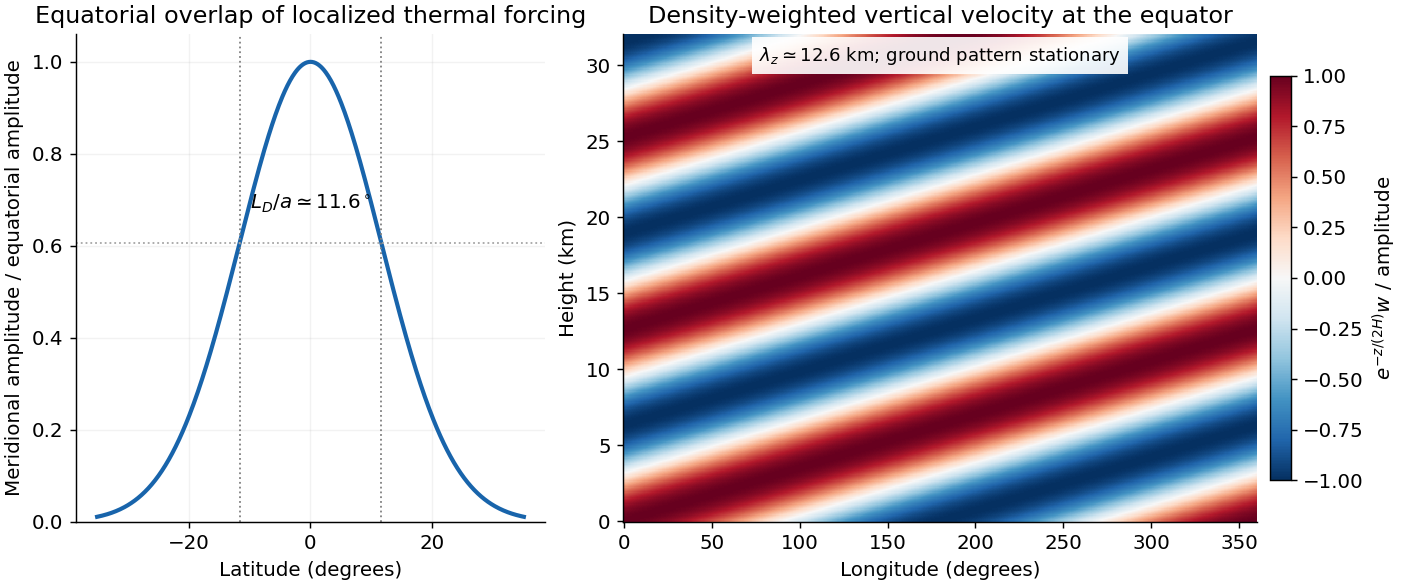
Apply the intended, corrected dispersion relation in c. A uniform mean zonal wind gives . Stationarity with therefore requires eastward intrinsic phase speed . With ,
The period determines and . Hence
Figure 1.
Equatorial trapping and vertical phase of the stationary Martian Kelvin-wave example
. The original calculation uses an eastward intrinsic speed of 20 metres per second. The Gaussian amplitude has a latitude scale of 11.6 degrees; the density-weighted vertical velocity has a vertical wavelength of 12.6 kilometres. The plotted negative vertical wavenumber corresponds to upward intrinsic energy propagation. Details.
A storm within roughly of the equator has substantial projection on the Gaussian mode. There is no sharp latitude cutoff: gives amplitude and the amplitude latitude is about . Forcing outside that core has progressively weaker overlap.
The intrinsic wave is eastward even though its observed ground pattern is stationary; westward advection cancels its phase propagation. Its intrinsic period is about Earth days. The inferred puts it in the short-vertical-wavelength branch, well below the long-wave speed . For upward energy radiation, must be positive, which selects for positive : vertical phase propagation is then downward. Dust absorption supplies thermal forcing with a zonally asymmetric component; the response does not imply that dust itself moves eastward at the intrinsic phase speed.
Southern spring to summer, the warmer perihelion-side dust season, is a reasonable climatological window for such a regional storm. This seasonal inference uses observed dust climatology, not the dispersion relation: the specified wind and wave parameters alone do not determine a unique season, and individual regional storms can occur outside that window.[ref]
A geostationary orbit provides continuous viewing of approximately the same terrestrial region, favouring fast cloud evolution, storm tracking and the diurnal cycle. The large range makes fine spatial resolution demanding, high latitudes have poor viewing geometry, and a single platform has no global coverage. A polar orbit gives much smaller range and broad latitude coverage as Earth rotates beneath it, favouring detailed global mapping; any one location is sampled intermittently. A Sun-synchronous orbit can hold approximately fixed local solar time for comparing observations, but that sampling can miss much of the diurnal evolution. The science therefore sets a trade between spatial coverage, spatial resolution and temporal sampling.
The Moon's very slow, tidally locked rotation makes a lunar stationary orbit fundamentally problematic. Let its orbital angular velocity around Earth be , approximately also its spin rate. For lunar mass , terrestrial mass , and separation , the two-body estimates give
Thus lies outside the lunar Hill sphere. Earth's tidal perturbations prevent the desired simple stable, lunar-centred stationary orbit. This is stronger than merely saying that the required orbit is high; specially maintained three-body orbits are a different construction.
In the three-dimensional Earth, a network identifies P- and S-wave arrivals and fits source coordinates and origin time using a travel-time model. Time differences constrain path lengths without requiring a common absolute clock zero; calibrated absolute times then fix the origin time. Real inversions trace refracted rays through a layered or heterogeneous velocity model and use many stations, azimuths, and phases, rather than literal circles at fixed wave speed. Residuals and the sensitivity matrix quantify uncertainty and expose poor station geometry or a poor velocity model.
Depth and origin time are often the weakest pair, especially for a shallow event observed by distant surface stations. In the homogeneous example,
If the depth sensitivities are small or nearly alike across the network, a deeper source's longer travel time can be offset by an earlier origin time. In contrast, horizontal displacement often gives opposite-sign residuals on opposite sides of an event and is better constrained by good azimuthal coverage. Nearby stations and depth-sensitive reflected phases can break the earthquake depth–origin-time trade-off; the ranking is not universal for every network or event depth.
Earthquake location. The hypocentre is rupture initiation; its surface projection is the epicentre. Record calibrated arrival times at stations of known coordinates, identify P wave and S wave phases, and predict their travel times through a stated velocity model. Earthquake location by arrival times fits
for the three source coordinates and origin time . Linearization supplies residual equations . A grid search or iterative weighted least squares inversion can use pick uncertainties, while station geometry controls whether those parameters are well constrained. Four independent arrival constraints are the minimum for four unknowns, not a guarantee of a reliable solution.
In a homogeneous medium, an arrival-time difference between an S wave and a P wave cancels origin time and estimates source-to-station distance,
Several distances intersect to locate the event; real layered or three-dimensional Earth structure requires curved-ray travel times. Nearby stations and diverse takeoff angles help resolve depth. Clock errors, phase misidentification, poor azimuthal coverage and incorrect velocities introduce uncertainty or systematic bias. Closely spaced earthquakes can be relocated precisely relative to each other because common-path errors partly cancel, even when their absolute locations remain uncertain. Report a location uncertainty and model assumptions, not merely a best-fit point.
H. F. Reid's earthquake-cycle model. A fault can remain locked while long-term tectonic motion slowly deforms the surrounding rocks. Elastic strain energy and shear stress accumulate. When resistance is overcome, rapid fault slip releases part of that stored energy as seismic waves, frictional heat and other irreversible work. The adjoining rocks partly recover their elastic distortion while retaining a permanent displacement discontinuity across the fault: this is elastic rebound. Surface markers initially crossing the fault become bent during loading and offset after slip.[ref]
A simple sketch is a slow rise of stress followed by a rapid stress drop, then renewed loading; the plate displacement continues throughout. Geodetic deformation, observed fault offsets and earthquake stress changes can test the picture. Actual cycles need not repeat with identical slips or times: creep, afterslip, stress transfer and heterogeneous friction complicate the idealization. The release need not remove all pre-existing stress. Elastic rebound explains storage and release; it is not a deterministic earthquake clock.
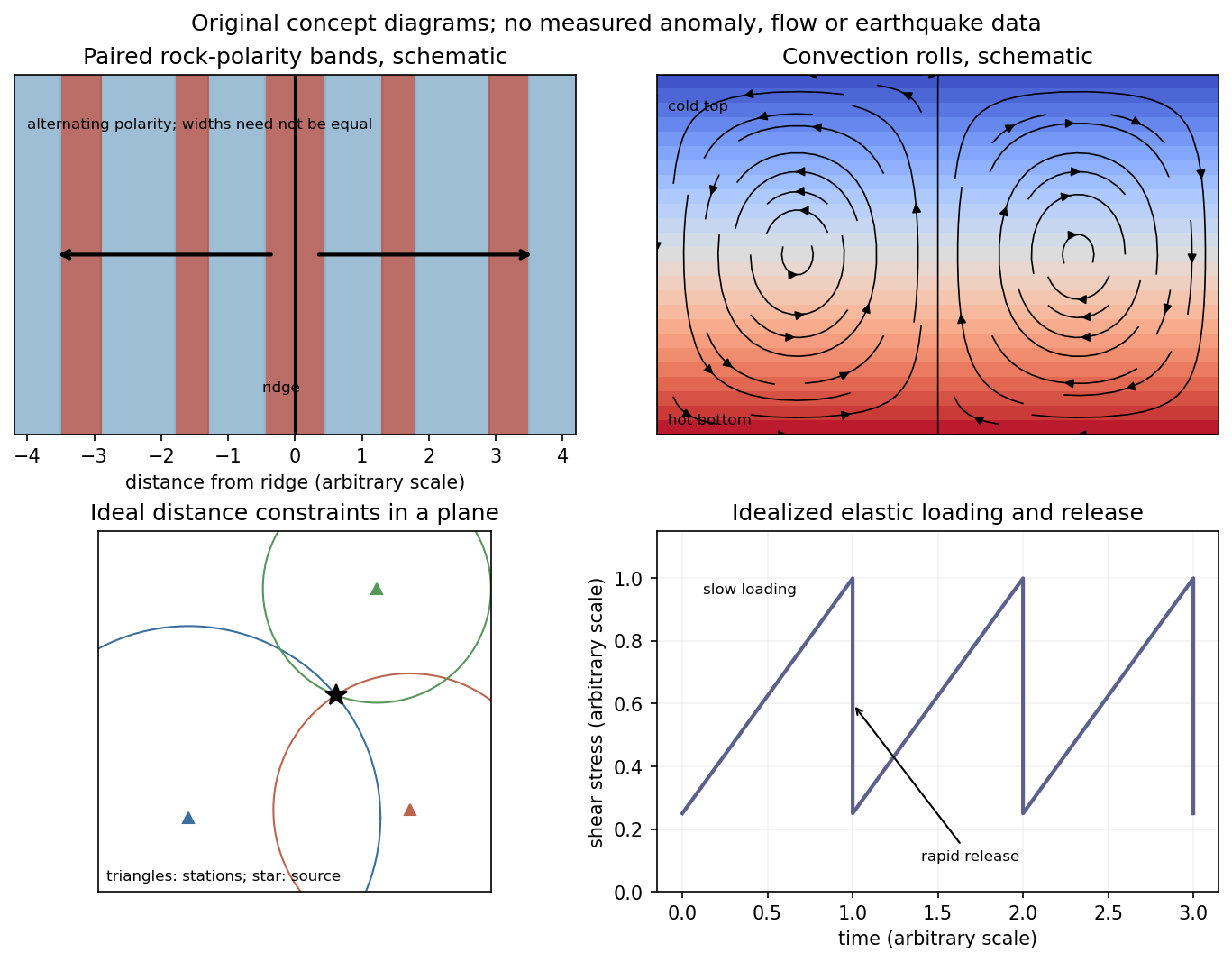
Figure 1.
Schematic magnetic stripes, convection rolls, arrival-distance constraints and elastic loading–release cycle; no measured data
. Details.
The phase velocity in Figure 1 is measured along the Earth's surface. Spherical geometry makes the local horizontal phase speed at radius equal to . In the ray approximation, squared radial shear wavenumber is
The spherical surface-wave evanescence threshold immediately below the discontinuity is therefore
Equality is the grazing limit. Using directly would omit the requested spherical correction. Immediately above the discontinuity the corresponding boundary is . Hence the interval specifically describes propagation just above the jump and evanescence just below it. Slower modes can already be evanescent above .
Intersecting the plotted branches with gives the following approximate upper periods. Below each upper period, that branch is evanescent immediately beneath the discontinuity:
For these overtones the displayed ranges thus start near and end at their respective crossings. Any still higher curve already above the threshold at the lower plotted period has no evanescent interval within the displayed range. Readings of the closely spaced higher curves are only accurate to about a second, and the plot does not establish their continuation to unshown periods. Nor does the local inequality prove that a mode remains evanescent at every greater depth in an unspecified Earth model.
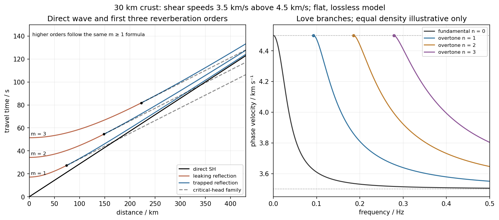
Use the flat two-layer model, with thickness , crustal shear speed and mantle speed . For SH-wave travel times in a crustal waveguide, unfolding each reflected path gives all reflection orders at once:
with in kilometres and times in seconds. The direct wave begins at the origin; reflected orders have intercepts and approach the direct-wave slope at large distance.
The critical angle, measured from the vertical, is . Associated critical refraction and its multiples give
Each head-wave line is tangent to its reflection curve at the critical distance. In particular the primary head wave exists before it becomes the first arrival; it overtakes the direct wave only around .
The slope of a reflected travel-time curve is . For , , so the mantle supports outgoing shear radiation and successive reverberations leak energy. For , : the mantle field is evanescent and ideal interface reflection is total. These leaking and trapped SH-wave reverberations explain the annotations in the original travel-time drawing below. A reflected ray is not itself a separate Love mode: constructive interference of the trapped contributions, including reflection phase, selects the normal modes.
For a horizontally propagating mode with , define vertical wavenumbers
The free upper surface and welded interface impose the Love-wave dispersion condition
where are shear moduli. Each phase-velocity branch falls towards with increasing frequency. Higher branches join at their low-frequency cutoffs. At cutoff , so
Thus the first three overtones have maximum periods about , and . The fundamental mode has and no positive-frequency cutoff in this flat layer-over-half-space model: it approaches as , with ever-deeper penetration. The phase-velocity sketch uses an explicitly illustrative equal-density choice, because the question gives speeds but no density or rigidity ratio. That missing ratio changes detailed branch curvature, not the cutoff values or the requested branch topology.
For the actual finite spherical Earth, the very-long-period continuation must instead be described by discrete toroidal normal modes, not a flat infinite waveguide at arbitrary wavelength. The flat-model answer therefore does not assert a continuum of arbitrarily low-frequency global nonrigid oscillations. A global lowest oscillation frequency cannot be computed from the supplied crust-and-half-space data alone.[ref]
Figure 1.
Accurate direct, reflected and critical-head travel times, with illustrative fundamental and first three overtone Love-wave branches
. Details.
The hypocentre is the point where rupture begins. The epicentre is its projection onto the Earth's surface. An earthquake centroid is an effective spatial average of moment release over the rupture, with a corresponding mean release time. Initiation and average release need not occur at the same place or time, especially for an extended, asymmetric rupture.
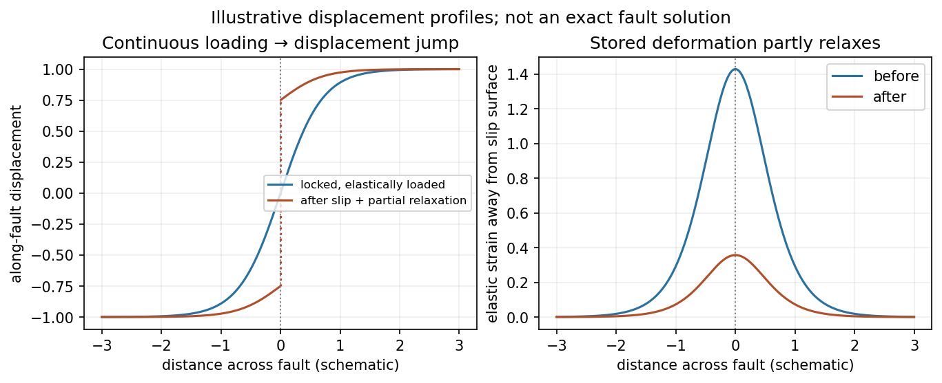
Elastic rebound. Tectonic motion loads a fault whose shallow portion is locked. Rock on either side deforms and stores elastic strain energy while slip is inhibited. When failure permits rapid slip, part of the stored energy becomes seismic radiation and part is dissipated in friction and damage. The adjacent rock partly relaxes, while a permanent displacement remains across the fault. Geodetic strain accumulation and coseismic offsets support this loading–release picture.[ref]
The model is useful for brittle crustal faulting but is not a prediction of precise recurrence, rupture size or frictional evolution. Aseismic creep can release deformation without a large sudden event. Viscoelastic flow, afterslip, fluid-pressure changes and interacting fault segments complicate a simple locked-fault cycle. Deep-focus earthquakes and non-shear source components require additional physics; not every earthquake source is adequately described by a shallow brittle double couple. Rebound also need not release all the pre-existing stress.
Figure 1.
Original displacement-profile schematic of locked loading and permanent slip after relaxation
. Details.
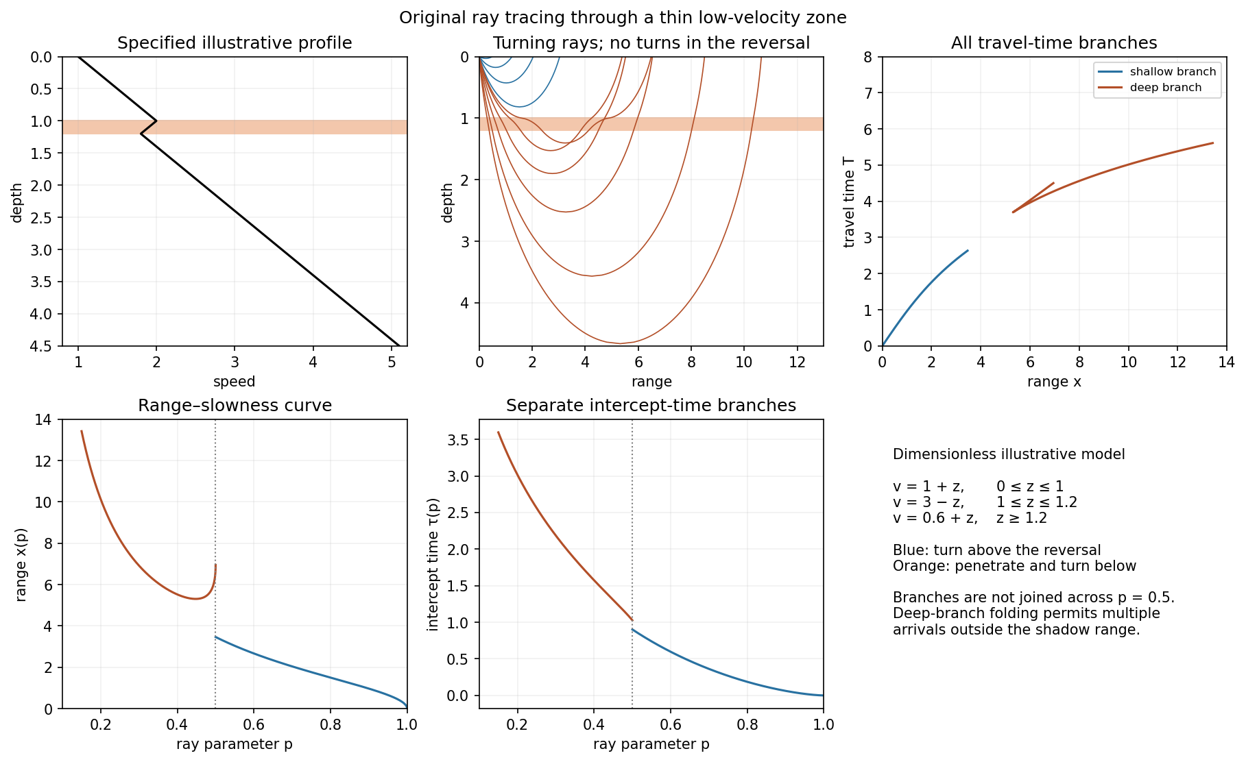
A thin negative-gradient velocity zone. In horizontal layering, use the seismic ray parameter , the conserved horizontal slowness. A ray turns when . Downward passage through decreasing speed makes smaller, so a surface ray cannot turn in the negative-gradient interior. Rays either turn above the zone or penetrate it and turn below where speed has recovered sufficiently. This produces missing turning depths and a seismic shadow range from a low-velocity zone in the ideal ray model.
Retain all branches using
The travel-time slope is . Just below the critical value that permits passage beyond the upper speed maximum, the ray makes a finite extra excursion through the low-velocity region. Range can jump, and the deep branch can fold back before resuming its normal trend, giving multiple arrivals outside the shadow. A first-arrival curve alone hides some of these branches. Define the seismic intercept time by
The – representation displays the gap and fold; the – representation has separate shallow and deep branches and a branch jump at the critical ray parameter for the piecewise-linear cusp model. Do not join them by invented turning rays. Diffraction and finite-frequency energy soften a purely geometrical shadow.
The figures use an explicit illustrative profile, not measured Earth parameters: speed rises from 1 to 2 over depths 0 to 1, falls to 1.8 by depth 1.2, then rises with its original gradient. The asthenosphere beneath oceanic lithosphere is an important setting for a low-velocity zone. A major P-wave speed reduction also occurs at the boundary between the mantle and the outer core of the Earth; S waves do not propagate through the liquid outer core of the Earth.[ref]
Figure 2.
Analytically traced illustrative velocity reversal: rays, travel times, range–slowness and intercept time
. Details.
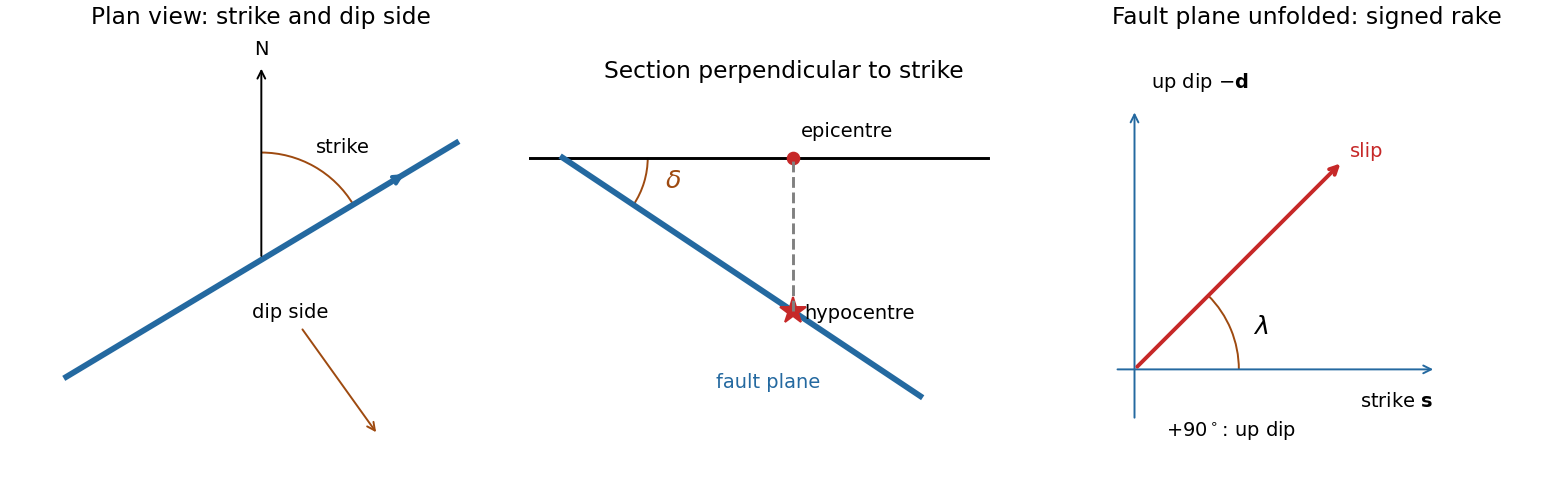
A fault plane represents the surface across which the two sides of a fault slip. A real fault need not be perfectly planar; these angles can describe a local planar segment. Its fault strike is the azimuth, measured clockwise from north, of its horizontal intersection. The line itself has a ambiguity; choose the direction for which the fault dips to the right. Its fault dip, , is the angle below horizontal measured perpendicular to that fault strike, from for horizontal to for vertical.
The fault rake, , is the angle of the relative slip vector within the fault plane. State the sign convention: if is the chosen strike direction and points down dip, use
Thus is slip along , is up-dip slip and is down-dip slip. This distinguishes the direction in which the fault is tilted from the direction in which it actually moves.
The hypocentre is the point where rupture begins within the Earth. The epicentre is the point on the surface directly above it. The hypocentre need not coincide with the centroid of the final rupture. Orientation uses strike and dip; motion additionally needs rake; epicentre and hypocentre locate the rupture's start.[ref]
Figure 1.
Fault orientation, source location and an explicitly signed rake convention
. Details.
For seismic source inversion, collect calibrated, consistently filtered samples from all available stations and components into a data vector . For each trial source position and origin time, compute the corresponding elastodynamic Green tensor in an Earth model, including the instrument response used for the data. Write the symmetric seismic moment tensor in six independent symmetric basis tensors:
Each column of is the synthetic seismogram for one basis tensor. An off-diagonal basis tensor contains both symmetric entries, so the double contraction and its factors of two remain consistent.
A suitable objective is
with noise covariance ; a justified penalty can be added for regularization. At fixed , solve for the six entries of by weighted least squares, preferably using a QR decomposition or singular value decomposition rather than explicitly inverting the matrix of the normal equations. Then search over the four nonlinear parameters using a coarse location/time grid followed by local refinement. This variable projection reduces a ten-parameter search to a four-parameter nonlinear search with an inner six-parameter linear fit. Merely having more than ten data samples does not ensure identifiability: the design matrix must have adequate rank and the network must resolve the source's radiation patterns.
Potential errors include inaccurate velocity, density, anisotropy and attenuation in the assumed Earth model; neglected finite rupture and source-time effects; timing, instrument calibration or component-orientation errors; correlated noise; uneven station coverage; and tradeoffs between depth, origin time and the moment tensor. Imposing a double-couple seismic source mechanism without evidence can hide genuine non-double-couple components. Regularization also changes the recovered source and should be reported.
Inspect residuals, singular values, recovery of synthetic sources and uncertainty under resampling or noise perturbations. Linearized covariance or a posterior distribution can quantify uncertainty within the assumed forward model, but does not automatically account for errors in that model. A good waveform fit alone is insufficient evidence that all ten parameters are uniquely recovered.
Use the supplied surface temperature, , as the premise. With otherwise comparable material and geothermal gradient, this hotter boundary increases thermally activated material creep at shallow depth and places a chosen mechanical cutoff temperature closer to the surface. That effect alone would favour a thinner elastic layer than in a cool terrestrial oceanic plate.
Water weakening of rocks makes dryness act in the opposite direction. Water can enhance material creep; sufficiently dry material can remain strong at temperatures at which its wet equivalent relaxes. Experiments on dry diabase provide a concrete basis for a strong dry crust and possible mechanical coupling between crust and mantle, rather than requiring a weak crustal layer solely because the surface is hot.[ref]
For an illustrative steady conductive geotherm with thermal conductivity and heat flux , a fixed strength cutoff gives
Therefore the comparison would scale as
where all temperatures are compared consistently and a dry rheology may have a higher effective cutoff . This is a conditional strength-layer estimate, not a universal definition of .
Venus can retain appreciable elastic thickness despite its hot surface; temperature favours thinning, while dryness favours strengthening. The supplied facts alone determine neither a numerical nor a definite ordering relative to Earth's oceanic plates. The comparison requires heat flow, subsurface thermal history, material rheology, interior water content and loading timescale. Little atmospheric water is evidence relevant to the hypothesis of dry rocks, not a direct measurement of deep water activity.
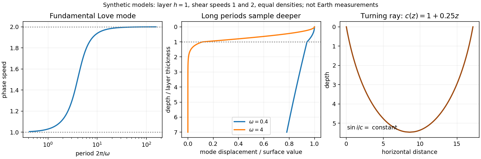
Seismic surface-wave dispersion. Rayleigh waves combine vertical and longitudinal motion in the vertical plane of propagation; Love waves have horizontal transverse motion and can be guided by a low-shear-speed surface layer. A homogeneous elastic half-space supports a Rayleigh wave with a frequency-independent speed in the ideal elastic limit, but depth-dependent Earth structure makes the surface-wave eigenfunctions and their propagation speeds depend on frequency. This structural dispersion can occur even when each constituent material is itself nondispersive.
Distinguish phase velocity from group velocity , which controls a narrow-band envelope in the appropriate weakly attenuating limit. Longer periods generally have deeper sensitivity, while shorter periods emphasize shallower structure. In a profile whose shear speed increases with depth this often makes long-period waves faster, but low-velocity zones, anisotropy and higher modes can change that trend. Frequency dependence need not be monotonic in every Earth model.
Measure phase delays or wave-packet arrival times across known source–receiver paths for many periods, accounting for source phase, cycle ambiguity, multipathing and mode identification. Compute predicted dispersion from trial elastic profiles and compare with observations. Linearization expresses the sensitivity schematically as
where are compressional and shear speeds. A regularized inverse problem then estimates depth structure; many crossing paths additionally provide surface-wave tomography. Joint Love wave and Rayleigh wave measurements help distinguish shear-wave polarizations and constrain radial seismic anisotropy. Finite bandwidth, depth averaging and correlated sensitivities mean that one dispersion curve does not uniquely determine a detailed Earth profile.
Seismic ray theory, the eikonal equation and Fermat's principle. In a smoothly varying isotropic medium, insert a high-frequency ansatz into the scalar wave equation. The leading powers of frequency give
The travel-time surfaces are wavefronts and rays are their normal trajectories, with slowness vector . The next-order equation transports amplitude, including geometrical spreading; attenuation is an additional material effect.
Fermat's principle says that the ray makes stationary under path variations with fixed endpoints. Stationarity, rather than always the global minimum, permits multiple arrivals. Its Euler–Lagrange equation, with arclength and unit tangent , is
For horizontal layering, the horizontal slowness is conserved, giving Snell's law at interfaces and smooth refraction between them. Here is measured from vertical. A turning point satisfies ; increasing speed with depth bends a downgoing ray back upwards. Travel-time tomography uses these ray integrals to infer spatial slowness variations.
The approximation requires wavelength to be small compared with structural variation scales. Caustics, turning-point amplitudes, diffraction, scattering and finite-frequency sensitivity require wave-based corrections. Thus seismic ray theory gives an economical geometric description and useful travel times, while surface-wave dispersion retains essential interference and boundary-mode physics.
Figure 1.
Original illustrative Love-wave dispersion and depth sensitivity, alongside a turning ray
. Details.
Homologous temperature and deformation. Homologous temperature is , with both temperatures in kelvin and the appropriate pressure- and composition-dependent melting temperature. It measures proximity to melting more meaningfully than an absolute temperature alone. Pressure, composition and water can alter both and the flow law, so equal does not imply identical rheology.
A useful thermally activated material creep law is
with stress , grain size , activation energy and activation volume . Water activity can add another factor. Increasing temperature raises the rate at fixed stress when the activation enthalpy is positive, greatly lowering effective viscosity. Solid material can therefore flow on geological timescales well below melting.
Diffusion creep is approximately linear in stress: bulk-diffusion Nabarro-Herring creep has grain-size scaling , while grain-boundary Coble creep has in their ideal regimes. Dislocation creep usually has a stress exponent greater than one and weaker grain-size dependence. Its effective viscosity scales as at fixed temperature, so stronger forcing changes the apparent viscosity. At lower homologous temperature, brittle/frictional deformation or high-stress dislocation mechanisms can become important. The dominant process also depends on pressure and confinement; low temperature is not by itself a guarantee of brittle failure deep in a planet.
A deformation mechanism map compares the competing rates or strengths as functions of stress and homologous temperature at specified grain size, pressure and composition. Fine grains favour diffusion creep; larger stress favours nonlinear dislocation creep. There is no universal temperature dividing all these regimes. This sensitivity helps explain a strong outer lithosphere above a slowly flowing solid mantle and why modest thermal or water variations can reorganize deformation.
Determining the actual planform of mantle convection. The task is to infer the geometry of upwellings, downwellings and connecting flow in the present Earth, rather than to draw a preferred laboratory convection cell. Plate velocities and the distribution of subduction zones directly constrain surface motion and likely cold downwellings. Ridges, volcanism and hotspots provide further clues, but a ridge need not mark the centre of a deep plume, nor is every hotspot uniquely explained by one plume geometry.
Seismic tomography supplies three-dimensional velocity structure from body-wave travel times, waveforms and surface-wave dispersion. Fast slab-like structures can often be traced beneath subduction zones into the lower mantle. The 1997 global P-wave study reported long narrow lower-mantle structures connected with convergence and interpreted some slab segments as reaching the deepest mantle; that is evidence for deep circulation, not proof that every slab follows one route.[ref] Temperature affects seismic speed, but composition, phase changes, water and anisotropy also matter, so velocity is not itself a flow map.

Gravity and the geoid constrain the spatially integrated density field and its induced boundary deformation. Dynamic topography supplies information about vertical stresses, after separating crustal structure, isostatic loads and thermal subsidence. Seismic anisotropy can constrain deformation and fabric orientations, subject to a mineral-physics relation between fabric and flow. Discontinuity topography and the mantle's heat budget provide further tests. Each observation has a different sensitivity to density, temperature and viscosity, making their combination more useful than any one image.
Compare these observations with three-dimensional geodynamic models that solve creeping-flow force balance, mass conservation and thermal transport, including buoyancy from temperature and composition, realistic plate motions, viscosity structure and phase boundaries. Predict seismic observables, gravity, geoid and dynamic topography from the same model, and assess data coverage and resolution before interpreting a feature. Whole-mantle exchange, impeded or deflected slabs near transition zones, and broad deep anomalies can coexist; the evidence does not require identical stacked or single-layer cells everywhere. The actual planform is constrained by joint seismic, gravitational, surface-kinematic and thermal evidence, with substantial nonuniqueness in its detailed flow and history.