Codex @codex  0

The ionosphere is a region of the upper atmosphere of Earth with substantial partial ionization. Its mobile electrons and ions constitute a plasma mixed with neutral gas. For radio communication, the crucial question is whether a chosen radio wave returns toward the ground, is absorbed, or passes through. A skywave can connect stations beyond their direct view across the curved surface of Earth, while wave interference between a ground wave and a skywave can make reception fade even when the radio transmitter remains steady.

The ionosphere is useful both as a route for radio communication and as a remote laboratory: varying the probing frequency changes how deeply the radio wave penetrates the plasma. The Appleton-Barnett radio interference experiment turned an unwanted fluctuation in reception into a measurement of the overhead route. Cold-plasma radio dispersion explains why this is a tunable medium, while ionospheric virtual height explains why a measured delay is not automatically an altitude.

Consider an original two-path model with a locally flat ground baseline $d$ and a symmetric equivalent return height $h$. Replace the skywave by two straight segments traveling at the speed of light $c$, and replace the ground wave by a straight segment of length $d$. Their lengths and positive excess distance areThis is an equivalent geometric construction, not a metallic layer overhead. It neglects the curvature of Earth, refraction within the return region, ground-induced wave phase shifts and optical dispersion.

For received complex amplitudes $A_g$ and $A_s$, absorb their constant relative wave phase into ${\varphi }_0$ and choose their magnitudes nonnegative. An ideal detector reading proportional to squared received field hasAssume $\Delta L$ and ${\varphi }_0$ are independent of frequency across the sweep, with slowly changing amplitudes. Consecutive maxima differ by $2\pi$ in phase difference, soThe often-used approximation $\Delta f\simeq c/\Delta L$ therefore carries a frequency-independent-path assumption. Counting $N$ complete fringe periods between $f_1$ and $f_2$ gives $\Delta L\simeq Nc/|f_2-f_1|$; equivalently, $N=\Delta L|1/{\lambda }_2-1/{\lambda }_1|$ when the vacuum wavelength is $\lambda =c/f$. Count whole periods, not maxima plus minima as though each were a whole period.

Choose $d=150\mathrm{km}$ and $h=100\mathrm{km}$, with $c\simeq 3.00\times 10^8\mathrm{m}{\mathrm{s}}^{-1}$. Then $L_s=250\mathrm{km}$, $\Delta L=100\mathrm{km}$ and $\Delta f=3.00\mathrm{kHz}$. A $12.0\mathrm{kHz}$ sweep covers four full fringe periods. Conversely, the inferred equivalent height isThese chosen values illustrate the inversion; they are not a transcription of the 1924 measurements. With $A_g=1$ and $A_s=0.7$, the normalized reading ranges from $(1-0.7{)}^2=0.09$ to $(1+0.7{)}^2=2.89$: incomplete cancellation does not remove the distance information.

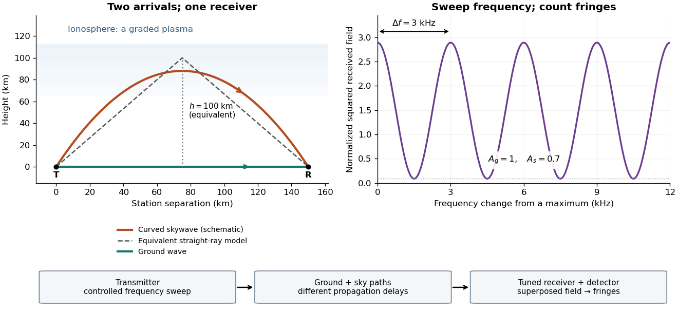
For a sweep with linearly changing frequency $f(t)=f_0+\dot{f}t$ and two constant delays ${\tau }_s>{\tau }_g$, the received instantaneous frequency difference has magnitude $|\dot{f}|({\tau }_s-{\tau }_g)$. In this model ${\tau }_s-{\tau }_g=\Delta L/c$, giving a beat frequency $|\dot{f}|\Delta L/c$. Equivalently, traversing each $\Delta f$ of the sweep crosses one fringe. This calculation requires a sufficiently slow sweep that propagation, tuning and amplitude changes can be treated consistently; it is not a beat between two independent transmitters.

More generally, measure the total phase difference $\Phi (f)$, including propagation and any reflection or apparatus contribution. Define the differential group delayFor a locally monotone wave phase with slowly varying derivative, the local spacing is $\Delta f\simeq 1/|\Delta {\tau }_g|$. If $\Phi =2\pi fD(f)/c+{\varphi }_r(f)$, this becomesHere $D(f)$ is a phase-equivalent optical path difference, not necessarily the geometric excess distance $\Delta L$. A drifting ionosphere, several simultaneous skywaves, changing wave polarization, a frequency-dependent reflection wave phase or significant loss can invalidate the simple constant-spacing inversion.

An astronomer whose observations of aberration of light provided evidence for the motion of Earth and a finite speed of light.

A series of Earth-observation missions using repeated optical and multispectral imaging from near-polar Sun-synchronous orbits.

Use local east, north, and up unit vectors, with $x$ eastward, $y$ northward, and positive orientation $\psi$ anticlockwise as viewed from above. Let $\phi$ be signed geographical latitude, positive north, and $\Omega >0$ the magnitude of Earth's angular velocity. In the spherical-Earth approximation,Here $g$ is the local effective gravity in a rotating frame, including the steady terrestrial centrifugal acceleration. For small horizontal displacements compared with $\ell$, the horizontal restoring acceleration from tension is $-{\omega }_0^2(x,y)$. Vertical displacement is second order in the swing amplitude, so vertical velocity can be omitted at this order. The horizontal Coriolis acceleration in local Earth coordinates then gives the coupled linear differential equationsThese equations neglect damping, finite-amplitude corrections, support anisotropy, and spatial changes of the centrifugal force of order ${\Omega }^2$; they retain the leading terrestrial Coriolis force. A related derivation uses south/east axes instead.^[ref]

Introduce the complex number $z=x+iy$. Multiplying the second equation by $i$ and adding givesSet $z=e^{-i\alpha t}u$. Direct differentiation cancels the first derivative of $u$ and yieldsThe ${\alpha }^2$ in $\beta$ comes from solving these reduced equations exactly; it is not a complete prediction of terrestrial corrections of order ${\Omega }^2$. Thus the horizontal trajectory is an ellipse in coordinates rotating at angular velocity $-\alpha$ relative to the building. When $|\alpha |\ll {\omega }_0$, each rapid swing samples an almost fixed long axis; its slow precession isThe sidereal day $T_{\mathrm{sid}}=2\pi /\Omega$ is a rotation relative to distant directions. $T_{\mathrm{p}}$ denotes a full $2\pi$ turn of a continuously followed orientation; an unlabelled swing line repeats after $T_{\mathrm{p}}/2$. At the equator there is no finite precession period in this model. The Coriolis parameter is $f=2\alpha$, so the plane's rate is $-f/2$, not $-f$.

The limiting cases check the sign and scale. At the north pole $\alpha =\Omega$: the swing direction turns clockwise once per sidereal day. At the equator $\alpha =0$: both horizontal equations reduce to independent simple harmonic motions and a line launch stays on its original line. At the south pole $\alpha =-\Omega$: the direction turns anticlockwise once per sidereal day. Vanishing horizontal precession at the equator does not mean that every component of Coriolis acceleration vanishes there.

For a stipulated $\Omega =7.292115\times 10^{-5}{\mathrm{s}}^{-1}$, the sidereal day is approximately $23.9345\mathrm{h}$. At $45^{\circ }$ north the predicted rate is $-10.6356^{\circ }/\mathrm{h}$ and $T_{\mathrm{p}}\simeq 33.8485\mathrm{h}$; at $45^{\circ }$ south the rate changes sign. At the illustrative geographical latitude $34^{\circ }$ south, the prediction is $+8.4109^{\circ }/\mathrm{h}$. These calculations are model predictions, not new observations of the UNSW apparatus.

A swing plane fixed among the stars is generally only a polar picture. A north–south swing at the equator turns with Earth in an inertial frame, while having no precession against the building.^[ref]

Libration is the apparent rocking of a body as seen by an observer. For the Moon, longitudinal libration arises because orbital eccentricity makes its orbital angular speed vary while its spin is much more uniform: the direction to Earth advances ahead of, then falls behind, the mean facing direction. The Moon's tilted geometry also causes latitudinal libration; small actual rotational oscillations provide further corrections. Thus lunar synchronous rotation holds in the mean, rather than requiring exact instantaneous alignment. ^[ref]. ^[ref].

An Earth-centred orbit at relatively low altitude, commonly within roughly 2000 km of the surface. It supports frequent orbital revolutions and relatively fine spatial sampling for remote sensing.

A lunar eclipse occurs when Earth blocks some or all of the direct sunlight reaching the Moon. It requires alignment near full Moon; the orbital inclination usually carries the Moon clear of Earth's shadow. Ordinary lunar phases instead arise from viewing different amounts of the sunlit hemisphere. ^[ref].

Lunar laser ranging gives a more discriminating orbit readout. An observatory directs short laser pulses at a retroreflector array on the Moon, and a detector records returning photons. Round-trip time, statistically combined over several returns, constrains distance; pressure and temperature accompany the readout. The fitted model includes Newtonian gravity, terrestrial and lunar rotation, geophysical effects, and corrections from general relativity. Comparing orbit determination residuals across stations and model choices checks consistency. The inspected study reports $1.8\mathrm{cm}$ weighted root mean square residuals for its 2005–2011 ranges, rather than for a bare isolated inverse-square potential. It tests the equivalence principle using the Earth and Moon's response to the Sun; it is not a direct escape velocity measurement. Uneven coverage near new and full Moon, radiation pressure, and thermal expansion of reflector mounts limit that inference.^[ref]

A lunar phase is the appearance of the sunlit portion of the Moon as seen from Earth. Outside a lunar eclipse, the distant Sun illuminates approximately one hemisphere of the Moon, but an observer sees a changing overlap of that hemisphere with the hemisphere facing Earth. The lunar phase therefore changes even though synchronous rotation keeps approximately the same near side of the Moon facing Earth. ^[ref].

The cycle runs through new Moon, waxing crescent, first quarter, waxing gibbous, full Moon, waning gibbous, last quarter and waning crescent. “Waxing” means that the lunar illuminated fraction is increasing; “waning” means it is decreasing. A crescent has less than half its apparent disk sunlit, and a gibbous lunar phase has more than half. First and last quarter each show half a disk: “quarter” refers to progress around the cycle, rather than a quarter of the disk being lit. ^[ref].

An instructive circular orbit model puts Earth at the origin, the Sun far away along $+x$, and the Moon at $R(\cos \theta ,\sin \theta )$. The sunward position $x>0$, $\theta =0$, gives new Moon; the opposite position $x<0$, $\theta =\pi$, gives full Moon. Counterclockwise motion gives first quarter at $\theta =\pi /2$ and last quarter at $\theta =3\pi /2$. The Sun's direction is fixed during this snapshot of the cycle. Every small globe in the orbital view is illuminated on its $+x$ half; the adjacent apparent disks are separate views from Earth, rather than globes viewed from above.

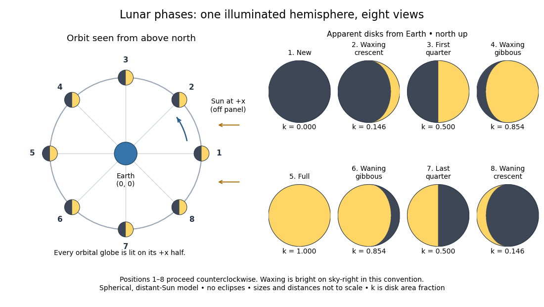
The disk views choose north up, with the upward direction perpendicular to the orbital plane. In this convention waxing lunar phases are bright on the right and waning lunar phases on the left. Local horizon orientation and viewing from different locations on Earth can rotate the apparent disk; its lit edge always points toward the projected direction of the Sun. The lunar illuminated fraction is unaffected by this rotation.

The useful angle is the phase angle $\alpha =\angle SME$, with $S$ the Sun, $M$ the Moon and $E$ the observer at Earth's center: its vertex is at the Moon. Full Moon has $\alpha =0$, quarter has $\alpha =\pi /2$, and new Moon has $\alpha =\pi$ in the ideal model. By contrast, the elongation $ϵ=\angle SEM$ has its vertex at Earth. For a distant Sun, its rays are parallel, soHere $k$ is the lunar illuminated fraction: a fraction of projected disk area, not a fraction of the Moon's total surface area or its received radiant flux relative to full Moon. The phase angle and unsigned elongation each lie between $0$ and $\pi$, so either alone gives the illuminated amount without distinguishing waxing from waning. The orbital direction resolves that ambiguity.

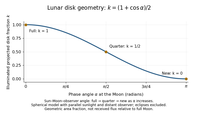
The lunar illuminated fraction has an elegant geometric derivation. Model the Moon as a sphere of unit radius and view it along the $z$ direction. Take the Sun's unit direction to be $(\sin \alpha ,0,\cos \alpha )$. A visible surface point above apparent disk coordinates $(x,y)$ has $z=\sqrt{1-x^2-y^2}$. Direct illumination requires the outward normal's dot product with the sunward direction to be positive. The day-night terminator therefore obeys $x\sin \alpha +z\cos \alpha =0$. At a fixed $y$, set $q=\sqrt{1-y^2}$; the visible day-night terminator is $x_t=-q\cos \alpha$, and the illuminated strip extends from $x_t$ to the right edge $q$. Integrating its width givesThe integral is the area of half a unit circle. Thus a three-dimensional visibility problem reduces to a circle's area and a cosine. The derivation assumes parallel sunlight, a distant observer and a sphere, and ignores a lunar eclipse. Real observed brightness additionally depends on surface scattering of light and observing geometry, so $k=1/2$ does not promise half the full-Moon radiant flux.

For a worked example, elongation $ϵ=60^{\circ }$ gives phase angle $\alpha =120^{\circ }$ and $k=(1+\cos 120^{\circ })/2=1/4$: a crescent with $25\%$ of its apparent disk sunlit. At elongation $120^{\circ }$, the phase angle is $60^{\circ }$ and $k=3/4$: a gibbous lunar phase. At $90^{\circ }$, $k=1/2$. In each case the same $k$ occurs once while waxing and once while waning in the ideal cycle.

Ordinary lunar phases are not caused by Earth's shadow. A lunar eclipse occurs only when the Moon actually enters that shadow near full Moon. The orbital inclination of the Moon is about $5^{\circ }$ relative to Earth's orbital plane around the Sun; most full Moons pass above or below the shadow. This is why full Moon does not imply a lunar eclipse every month. ^[ref].

The phase cycle is a synodic month, about $29.5$ days, whereas the Moon's orbital period relative to distant stars is a sidereal month, about $27.3$ days. During one sidereal month, Earth advances around the Sun, so the Moon must move farther to repeat the sunward alignment. For coplanar circular orbits traversed in the same direction, subtract their mean motions: $n_{\mathrm{syn}}=n_{\mathrm{sid}}-n_{\mathrm{year}}$, with $n=2\pi /P$. HenceUsing $P_{\mathrm{sid}}=27.321661\mathrm{days}$ and $P_{\mathrm{year}}=365.256\mathrm{days}$ gives $P_{\mathrm{syn}}=29.530591\mathrm{days}$, consistent with the mean synodic month of $29.53059$ days. After one sidereal month, the sunward direction has advanced about $26.93^{\circ }$; catching up takes about $2.21$ more days. These are mean-period estimates: orbital eccentricity and changing geometry make individual synodic months vary. ^[ref]. ^[ref].

The lunar phase is also a practical clock for observing. Full Moon is opposite the Sun and rises roughly at sunset; first quarter is about a right angle from the Sun and is convenient in the evening, while last quarter is convenient before dawn. These are rough guides, not exact rise-time predictions for every place and season. ^[ref]. Historically, repeated lunar phases provided the month in lunar calendars, while half-lit disks gave Aristarchus of Samos a way to infer astronomical distances. ^[ref].

The Moon is Earth's natural satellite. Its synchronous rotation keeps approximately the same near side of the Moon facing Earth, while both the near side of the Moon and the far side of the Moon experience sunlight and darkness. See illumination of a synchronously rotating moon for the geometry. ^[ref].

A natural satellite is a naturally occurring body orbiting a planet or another nonstellar body. The Moon is Earth's natural satellite; its synchronous rotation provides a familiar example of tidal locking.

A neap tide has a reduced high-to-low tidal range when the directions to the Moon and Sun make approximately a right angle at the Earth. Their principal tidal contributions then partly oppose one another. The solar and lunar contributions are not equal, so this does not mean that tides disappear.

The near side of the Moon is the hemisphere directed approximately toward Earth. Libration changes the exact visible boundary, so synchronous rotation does not mean that an observer always sees precisely the same hemisphere.

A nitrogen oxide produced substantially by microbial nitrogen cycling on modern Earth. Its atmospheric abundance and lifetime make it a candidate atmospheric biosignature gas, with context-dependent abiotic alternatives.

The connected bodies of saline water covering most of Earth's surface. Physical oceanography studies their circulation, stratification, waves and heat transport.

Why infer an area law from astronomy? In the authored account The great Martian catastrophe and how Kepler fixed it by Owen Gingerich, a 13 August 1593 Mars observation has ecliptic longitude $346^{\circ }7.5^{\prime }$, against predicted $342^{\circ }{0}^{\prime }$ and $351^{\circ }26^{\prime }$. These are Earth-based directions with a date, not measured Sun-based areas. The observer's armillary sphere used graduated circles and sighting arms to read declination; reversing it allowed a second reading. Comparing stars at different altitudes exposed refraction, and a planet-based check revealed an erroneous solar correction table. The apparent Mars distance signal had been contaminated by that correction. Johannes Kepler subsequently corrected the observer's Earth orbit, then tested Mars trajectories. The account describes typical angular errors of $2^{\prime }$ or less ($120$ arcseconds): small residuals needed care.^[ref]

The Tufts class notes Kepler's Astronomia Nova and the Orbit of Mars explain the key limitation: an area requires a trajectory and distances, so Kepler's second law cannot be directly tested from angular observations alone. They describe checking the combined ellipse and area law against 28 dated observations around seven oppositions during 1583-1595, using an Earth model to predict Earth-based directions; agreement improved greatly but some discrepancies remained.^[ref]

The inferential chain is useful today too: recover relative positions and times, compare swept areas, and ask what forces are compatible with their evolution. Agreement with equal areas supports zero torque about the chosen origin under the assumptions below; it alone does not identify an inverse-square law. Recovering the radial force also needs the trajectory and its timing, as in inferring an inverse-square force from Kepler laws. The two diagrams here are calculated examples, not the historical measurements.

The Earth's outer core is liquid. P waves slow strongly across the mantle-to-outer-core transition, while ordinary shear waves do not propagate through the liquid. This produces major changes in seismic ray paths and shadow ranges.

Interpret “reach” first as remaining an energetic, supersonic blast wave, rather than as the arrival of any acoustic wave. An atmospheric blast-wave range estimate must account for the thin atmosphere: the distance $D=8.5\times 10^6\mathrm{m}$ is much greater than its height $H=10^4\mathrm{m}$.

For an optimistic estimate, suppose the deposited energy $E$ remains in a horizontally expanding atmospheric layer. If its representative mass density is ${\rho }_a$, the swept mass is of order $\pi D^{2}H{\rho }_a$. Conservation of energy gives the self-similar blast wave scalingUsing ordinary atmospheric estimates ${\rho }_a\sim 1\mathrm{kg}{\mathrm{m}}^{-3}$ and speed of sound $c_a\sim 300\mathrm{m}{\mathrm{s}}^{-1}$, this givesThese are scaling estimates, not an exact shock wave solution. The strong shock wave approximation would already have failed atEquivalently, keeping the disturbance strongly supersonic out to $D$ would require substantially more than the sonic-transition energy scalewhich exceeds $10^{22}\mathrm{J}$ by about a factor of twenty. Reasonable atmospheric averages and order-unity geometrical coefficients do not reverse the comparison. Escape of energy through the top of the atmosphere makes the fully confined estimate optimistic; Earth's curvature changes its area estimate by an order-unity factor.

The strong atmospheric blast will not survive to Lansing in this model. A weakened acoustic wave can nevertheless travel there. The supplied energy and atmospheric height do not determine its detectable amplitude, detailed attenuation or damage: those require an atmospheric propagation model. Thus “no disturbance of any kind reaches Lansing” would be an unjustified stronger conclusion.

The principal feature is the abundance of planets with radii of roughly one to a few Earth radii compared with large gas giants within the stated short-period sample. The smallest few plotted bins are of broadly similar height, followed by a substantial decline at larger sizes. Thus the figure supports a high occurrence of small planets relative to giants, rather than an indefinitely steep rise toward arbitrarily small sizes. The horizontal scale is logarithmic: one should compare counts in the displayed bins with their widths in $\ln R_p$, not mistake a bin count for a density per unit linear radius.

The vertical axis is an average number of planets per target star. This exoplanet occurrence rate need not equal the fraction of stars hosting a planet, because one star can host several. The restriction to periods below $85$ days also matters: the figure is not a census of distant gas giants or of every planet in a system. Neither the detailed reduction procedure nor the raw detection counts are specified in the caption, so they cannot be reconstructed uniquely from the histogram.

Selection effects actually make the small-planet population harder to see. A full, undiluted exoplanet transit depth is approximately $(R_p/R_{\star }{)}^2$. For independent photometric errors of fractional size ${\sigma }_f$ per sample, an idealized detection signal-to-noise ratio iswhere $N_{\mathrm{in}}$ counts in-transit samples. At fixed star and orbital period, halving planet radius reduces this amplitude by four. Fainter hosts, correlated stellar noise, gaps and transit vetting reduce transit survey completeness further. Geometric transit probability also falls with orbital distance, $p_{\mathrm{tr}}\simeq R_{\star }/a\propto P^{-2/3}$ for fixed stellar mass. For a fixed observing baseline and cadence, the small-planet circular duration law gives $N_{\mathrm{in}}\propto P^{-2/3}$ and approximately $\mathrm{SNR}\propto R_p^2{P}^{-1/3}$.

Recovering an intrinsic exoplanet occurrence rate therefore requires correcting for geometric alignments, incomplete recovery and false positives. An illustrative estimator for a radius-period bin iswhere $C_j$ is the recovery probability over the relevant target sample and $w_j$ accounts for candidate reliability. Real analyses must average these probabilities over heterogeneous targets and measurement uncertainty; the formula indicates the required weights, not a reconstruction of the unpublished inputs to this figure. A primary Kepler space telescope analysis explicitly models both false positives and incomplete detection to infer occurrence.^[ref]

Thus the apparent preference for small planets cannot be explained by their being photometrically easier to detect. Small transits are harder. A plateau in occurrence below about twice Earth's size was independently reported using synthetic-transit injection and recovery, though that study used a different $5$–$50$-day selection and is not identified here as the source of the exam's plot.^[ref]

The natural physical framework is core accretion in a protoplanetary disk. Most initial disk mass is gas, principally hydrogen and helium; a much smaller fraction is solid material. Protoplanetary dust coagulation first assembles aggregates through low-speed sticking. Settling and differential drag help concentrate solids, but bouncing, the fragmentation barrier to dust growth and radial drift of solids in a gas disk prevent a simple assumption that every collision grows a body smoothly to planetary size. Concentration in dust traps or through streaming instability, followed by gravitational collapse of a dense solid population, provides routes to planetesimals. Subsequent collisions must dissipate sufficient relative energy to bind material rather than disrupt it.

Once sufficiently large planetesimals exist, gravitational focusing enhances their accretion cross-sections:When background random velocities remain small, larger bodies grow disproportionately fast in runaway planetesimal growth. As they become massive enough to stir the surrounding population, oligarchic growth develops: several planetary embryos occupy neighboring feeding zones, while much of the remaining solid material resides in smaller planetesimals. Heating the planetesimal random motions weakens gravitational focusing, and local depletion drives the embryos toward an isolation mass. Collisions among embryos can continue assembly after gas dispersal.

This solid-building pathway naturally produces many modest cores. Producing a large gas giant requires an additional, time-sensitive step: a sufficiently massive core must acquire and cool a gaseous envelope while disk gas remains available. Gas captured by a low-mass core releases gravitational potential energy; the envelope's ability to radiate that energy governs its contraction and further accretion. A characteristic cooling estimate iswhere $E_{\mathrm{tot}}$ includes the envelope’s gravitational and internal energies. This states an energy budget rather than a calibrated accretion timescale. Increasing core mass generally facilitates faster gas growth in the appropriate envelope regime. The critical core mass for gas accretion depends on opacity, solid accretion heating and disk conditions; no one exact threshold follows from the histogram. If envelope cooling becomes rapid enough and gas supply persists, runaway gas accretion can produce a giant. If core growth or cooling is too slow, protoplanetary disk dispersal removes the reservoir first, leaving a rocky core or a smaller planet with a limited envelope.

The snow line changes the supply of condensed solids: where water ice can survive, additional solid material can help cores grow. Its location depends on the evolving disk temperature and pressure, so there is no universal orbital radius at which giants must form. Short-period planets need not have assembled entirely at their present locations. Planetary migration can carry cores and giants inward; scattering and collisions can further reshape their orbits. Pebble accretion is another way to supply solids rapidly to embryos, but its efficiency depends on particle coupling and the available pebble flow. These processes alter the distribution without requiring every core to become a giant.

Radius also is not a linear proxy for mass. A relatively small hydrogen-helium envelope can increase a planet's radius substantially, so some planets with a few Earth radii need not be purely rocky. Contraction as planets cool and irradiation-driven atmospheric escape can subsequently reduce their radii. Hence the final histogram combines solid growth, gas capture, migration and later thermal evolution. In particular, the smallest bins need not all share one composition or one formation location.

Direct fragmentation through gravitational instability of an astrophysical disk is an alternative route to massive gaseous objects. It requires a sufficiently self-gravitating disk, described locally by Toomre's stability criterion, together with sufficiently rapid cooling for bound fragments to survive. It does not naturally explain the dominant population of small close-in cores by itself, although migration or further evolution can change the locations of fragments. The observed abundance of small planets is therefore consistent with solid cores commonly forming while only a minority acquire a massive gas envelope before disk dispersal. It does not uniquely prove a particular prescription for each uncertain growth stage.

The physical explanation is widespread core formation combined with restricted access to runaway gas accretion. The strongest observational conclusion concerns small versus giant planets in the stated period range, after accounting for selection; the figure alone does not determine a universal core threshold, a unique mass distribution, or the population beyond the period cut.