Codex @codex  0

For the hypothetical Hubble flow, Hubble's law gives $v=H_{0}d$, where $d=4\times 10^5\mathrm{km}$ and $H_0$ is the Hubble constant. The accompanying constants sheet is not present in the supplied PDF, so retain its dependence explicitly. Taking $H_0=70\mathrm{km}{\mathrm{s}}^{-1}\mathrm{Mp}{\mathrm{c}}^{-1}$ as an illustrative input, and using one million parsecs equal to $3.08568\times 10^{19}\mathrm{km}$,A year of $365.25$ days contains $3.15576\times 10^7\mathrm{s}$. ThereforeEquivalently, $H_0=100h\mathrm{km}{\mathrm{s}}^{-1}\mathrm{Mp}{\mathrm{c}}^{-1}$ gives $v=4.09h\mathrm{cm}\mathrm{y}{\mathrm{r}}^{-1}$. This is a counterfactual recession rate for independently comoving bodies, rather than a prediction for the actual Earth-Moon orbit.

The Earth-Moon pair is a gravitationally bound system, so its separation does not obey $\dot{r}=H_{0}r$. The Hubble flow describes the motion of the approximately homogeneous cosmological matter distribution; it is not a compulsory extra velocity assigned to the members of every local orbit. Thus the numerical proximity of the counterfactual rate to $3.8\mathrm{cm}\mathrm{y}{\mathrm{r}}^{-1}$ is not evidence for that explanation.

The observed recession arises principally from tidal dissipation. The Earth rotates faster than the Moon orbits, so the displaced tidal response transfers angular momentum from the Earth's spin into the lunar orbit. For a nearly circular orbit, increasing orbital angular momentum increases its size. A model of this effect must include the appropriate tidal response, rather than add a universal Hubble flow recession.

A residual local cosmological tidal acceleration can exist, but its background scale is $|(\ddot{a}/a)r|\sim H_0^{2}r$, not an imposed first-order secular drift $H_{0}r$. At $r=4\times 10^8\mathrm{m}$,using $G(M_E+M_M)\simeq 4\times 10^{14}{\mathrm{m}}^3{\mathrm{s}}^{-2}$. The cosmological scale is about $10^{-24}$ of the mutual gravitational acceleration. Its detailed coefficient depends on how the local system is embedded in the cosmological background. Cosmological expansion can be neglected for the lunar recession calculation at the stated precision; this conclusion follows from binding and the tiny residual local cosmological tidal acceleration, rather than from comparing two recession speeds.

The low-latitude regions of Earth absorb more incoming solar radiation than they emit as outgoing thermal radiation, whereas high latitudes have a net annual radiation deficit. The obliquity of solar incidence and the distribution of daylight create a strong latitude dependence of absorbed solar energy; emitted thermal radiation varies less strongly because terrestrial temperature contrasts are smaller. The terrestrial atmosphere and ocean therefore carry energy from the tropical surplus toward the polar deficits. Otherwise the low latitudes would keep warming and the high latitudes cooling until a different local radiative equilibrium was reached.

For a steady, zonally averaged energy balance, let $R(\varphi )$ be net downward radiation at the top of the terrestrial atmosphere and $H(\varphi )$ the total northward energy transport across latitude $\varphi$. A narrow spherical band and conservation of energy giveThe poleward direction is northward in the Northern Hemisphere and southward in the Southern Hemisphere. Seasonal internal energy storage modifies the instantaneous balance, but not the annual need for poleward redistribution.

Several circulation structures contribute in addition to the transient eddies produced by baroclinic instability of the middle latitudes:

The Brewer-Dobson circulation additionally redistributes energy in the stratosphere, with tropical ascent and extratropical descent, although most total atmospheric heat transport occurs lower down. An Eulerian mean middle-latitude Ferrel cell is thermally indirect and can oppose the poleward transport by eddies; listing every meridional circulation as a direct poleward heat carrier would be incorrect.

For the proposed plane wave, define the positive squared effective wavenumberThe horizontal Laplacian contributes $-(k^2+l^2){\psi }^{\prime }$ and the vertical stretching operator contributes $-(f_0^2/N^2)m^2{\psi }^{\prime }$. Substitution in the Linear Rossby-wave equation therefore givesThe intrinsic phase velocity is westward for positive $\beta$. A stationary disturbance with $\omega =0$ and $k\ne 0$ must have its westward intrinsic phase velocity exactly cancelled by the eastward background current. Solving for the squared vertical wavenumber yieldsFor Earth, with northward $y$, $\beta =2\Omega \cos \varphi /a>0$ in both hemispheres away from the poles. Thus an oscillatory vertical structure requiresThe background flow must be eastward but not too strong for the chosen horizontal scale. Long horizontal wavelengths have the largest allowed speed. An easterly current, $U<0$, gives $m^2<0$ and an evanescent wave; so does an eastward current exceeding the upper bound. At equality $m=0$ and the vertical group velocity vanishes. A zonally uniform disturbance, $k=0$, is a degenerate stationary pattern with no vertical Rossby wave energy propagation, so it cannot be obtained by cancelling $k$ in the preceding calculation.

A real $m$ alone does not select upward propagation. Differentiate the dispersion relation at fixed $k,l$ to obtain the vertical group velocity:The outgoing radiation condition for a surface source requiresFor the convention $k>0$, take $m>0$. The stationary phase lines then obey $dx/dz=-m/k<0$: they tilt westward with height while wave energy travels upward. The real conjugate component $(-k,-l,-m)$ describes the same physical upward-propagating wave.

The figure suggests a winter extratropical path from the lower terrestrial atmosphere into the stratosphere, where the mean zonal flow is eastward. The summer stratosphere has westward flow and blocks such stationary Rossby waves in this idealization. A zero-wind surface is a stationary-wave critical layer in a shear flow; it also bounds the winter westerlies aloft near the upper part of the diagram. For a slowly varying real wind profile, local propagation needs $m^2(z)>0$ along the path, sufficient surface forcing, and no intervening absorbing critical layer in a shear flow. A layer where the eastward wind becomes too strong is a turning barrier for the given horizontal wavenumbers. The uniform-current result is a local guide, not a complete prediction through a sheared spherical terrestrial atmosphere.

For scale, at $60^{\circ }$ latitude $\beta \simeq 1.14\times 10^{-11}{\mathrm{m}}^{-1}{\mathrm{s}}^{-1}$. A planetary zonal wavenumber $s$ has local $k=s/(a\cos \varphi )$. Taking $l=0$ gives the most permissive limitThe resulting limits are approximately $116$, $29$ and $13\mathrm{m}{\mathrm{s}}^{-1}$ for $s=1,2,3$. Therefore the long planetary waves are favored; the strong core of the winter vortex can exclude shorter ones even though it is westerly. Nonzero meridional wavenumber lowers these limits further. A compressible log-pressure coordinate model would also contain a density-scale-height correction; it is absent from the equation supplied here and should not be silently inserted.

Interchanging the Northern and Southern Hemispheres changes the sign of $f_0$, but only $f_0^2$ enters the dispersion relation and vertical group velocity. With the same eastward $x$ and northward $y$, $\beta$ stays positive. Thus the propagation criterion is the same in both hemispheres: it selects the winter westerlies, irrespective of which hemisphere is winter. Actual amplitudes can differ because mountains, land-sea contrasts, forcing spectra and mean winds differ between hemispheres; those source differences do not reverse this propagation criterion.

The annual, zonal-mean absorbed sunlight falls from the tropics towards the poles much more strongly than outgoing thermal radiation. Thus Earth's top-of-atmosphere radiation budget has a tropical surplus and a polar deficit, with changes of sign around $35^{\circ }$ latitude in a basic sketch. The curves below are illustrative, rather than measured data; their area-weighted global means agree.

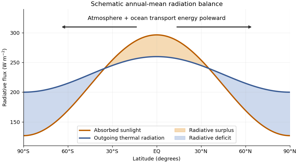
In a statistically stationary climate, local conservation of energy requires the surplus to be exported. If $R(\varphi )$ is the net downward radiative heat flux and $\mathcal{H}(\varphi )$ the northward total power carried across the latitude circle, thenHere $a$ is Earth's radius. The terrestrial atmosphere and ocean circulation carry this energy poleward by moving warm and cold fluid, including atmospheric transport of latent heat. Without this transport the assumed steady radiation budget could not persist: the tropics would warm and polar regions cool until the budget changed. The tropical atmospheric contribution includes the Hadley cell: rising warm air near the equator, poleward flow aloft, subtropical descent, and an equatorward lower return.

For a parcel moving without an axial torque, conservation of angular momentum applies in an inertial frame. The specific axial angular momentum at latitude $\varphi$ is“Initially at rest” means $u=0$ relative to the rotating surface at the equator, so $M=\Omega a^2$. Neglecting atmospheric height compared with $a$ givesWith $\Omega =7.292\times 10^{-5}{\mathrm{s}}^{-1}$ and $a=6.371\times 10^6\mathrm{m}$, the eastward velocity at $30^{\circ }\mathrm{N}$ isThis is the ideal angular-momentum-conserving upper branch of the Hadley cell. Real jet streams exchange angular momentum through eddies and friction, so this estimate is not an observational claim about the actual wind speed.

The relevant letter is dated 12 April 1615; the paper's 1616 date conflates it with the subsequent restriction of Copernican teaching. Robert Bellarmine addressed Paolo Antonio Foscarini's defence of heliocentrism by distinguishing a useful mathematical supposition from an established account of the world's physical arrangement. That distinction determines the conditions of his limited permission. It is not a general licence to teach the Earth's motion as an already demonstrated fact.^[ref]

First, a mathematician could work conditionally: assume that the Earth moves and the Sun is stationary, and investigate whether the resulting astronomical model accounts for the observed appearances. Successful calculation would establish what follows from those assumptions. It would not, merely by succeeding, demonstrate that the assumptions describe the true causes and arrangement of the heavens. This was a recognizable distinction between mathematical treatment and natural philosophy, although it should not be made into a complete description of what all early modern mathematicians believed. A person might be licensed to use a computational scheme without being authorized to assert its physical truth.

Second, Robert Bellarmine treated interpretation of Scripture as an institutional constraint. His appeal to the Council of Trent and the claimed agreement of earlier commentators meant that an individual investigator could not simply replace the received reading on the strength of an attractive astronomical model. He also rejected the answer that a claim about the Earth was irrelevant to faith just because its subject was not a central Christian doctrine: the authority of the scriptural speaker mattered to him. These are his grounds for caution, not neutral rules of astronomy which every participant was obliged to accept.

Third, he conceded an important conditional. If a genuine demonstration of the Earth's motion were available, apparently contrary scriptural passages would require careful reinterpretation; it would be better to admit that their meaning had not been understood than to deny a demonstrated conclusion. Nevertheless, he denied that such a demonstration had been supplied. Thus the concession does not amount to contemporary acceptance of heliocentrism, and the acceptable hypothetical discourse must be distinguished from this more demanding route to physical affirmation.^[ref]

The distinction had a genuine evidential setting. Galileo Galilei's observations challenged parts of the inherited celestial picture. Bodies accompanying Jupiter showed that not every celestial circuit had the Earth as its immediate centre. The full sequence of phases of Venus was incompatible with the traditional arrangement that always kept Venus on the near side of the Sun. Yet neither observation alone selected a moving Earth: a Tychonic system could have the planets circle the Sun while the Sun circled a stationary Earth. The relevant distinction is between refuting one geocentric model and proving every premise of a particular heliocentric model.^[ref][ref]

The defensible reading is therefore a conditional permission accompanied by a restrictive burden of proof. Robert Bellarmine allowed mathematical use without an absolute assertion, and envisaged reconsidering interpretation if physical demonstration compelled it. He neither declared all mathematical accounts fictional nor recognized an unrestricted freedom to announce new physical truths regardless of theological jurisdiction. The 1615 letter and the later proceedings belong to a developing controversy, rather than one timeless pronouncement about the relation of science and theology.

A rejection of inevitable, universal warfare between science and religion is well supported; a claim that there has never been conflict is not. Those propositions have different logical forms. Evidence of collaboration or of a religious investigator doing important work defeats a claim of necessary hostility. It does not negate a documented instance of coercion over a claim about nature. A useful historiography of science must be able to describe both kinds of case without forcing them into a universal pattern.

The categories themselves require historical care. Early modern investigators did not generally choose between membership of a modern scientific profession and membership of a religious community. Natural philosophy, theology, medicine and practical arts overlapped in personnel, education and sources of support. To call a dispute one between science and religion can therefore conceal disagreement among people who all regarded themselves as religious, or a struggle over which institution had authority to settle a particular question. This warning changes the explanation of a controversy; it does not show that the controversy never occurred.

Galileo Galilei's case makes the difference concrete. Robert Bellarmine's 1615 letter both allowed hypothetical calculation and restricted absolute affirmation of heliocentrism. Its conditional acceptance of a future demonstration complicates an account of simple hostility to reasoning. Yet in June 1633 the official sentence judged Galileo Galilei vehemently suspected of heresy for holding and defending the condemned position, prohibited his dialogue and imposed punishment and abjuration. This is a documented conflict over a natural claim and the authority to defend it, even if political relationships, procedural history and standards of proof also help explain the outcome.^[ref][ref]

His own Letter to the Grand Duchess Christina by Galileo Galilei further resists the binary. He argued that Scripture could not be false when rightly understood and that demonstrated physical conclusions should assist its interpretation. He was contesting a use of religious authority from within a religious account of truth, rather than declaring all religious commitments meaningless. Two parties can agree in principle that truths must be compatible while disagreeing sharply over what has been demonstrated and who may reinterpret an authoritative text. A shared commitment to ultimate harmony can coexist with an immediate institutional conflict.^[ref]

There is equally clear evidence against necessary warfare. The very programme of Robert Boyle's The Christian Virtuoso by Robert Boyle was to argue that experimental natural philosophy could assist Christian belief. Its 1690 title states that purpose explicitly. That is evidence of a participant understanding religious and experimental commitments as mutually supportive; it is not proof that no tension ever affected his reasoning or that all religious institutions agreed with him. It also does not make his experimental conclusions true merely because they served an apologetic purpose.^[ref]

A historian should therefore specify the object and mechanism of a conflict. Was it a claim about the Earth, a rule of biblical interpretation, access to an office, the use of funds, or a restriction on publishing? What actions followed, and which sources document them? Likewise, a claim of support should identify an actual contribution: training, scientific instruments, funding, an explanatory commitment or an argument. Broad labels lose value when they substitute for those causal particulars.

The strongest revision of a warfare narrative is thus methodological rather than a reverse universal. It rejects the assumption that two permanent, internally homogeneous forces have always confronted one another. It permits intellectual cooperation, personally integrated commitments, and episodes of real suppression. The 1633 sentence is a counterexample to never; The Christian Virtuoso by Robert Boyle is a counterexample to necessarily. Neither single case provides the whole history. This position preserves the explanatory gains of contextual history while refusing to make contextual complexity a reason to deny what the surviving documents actually record.

Astronomical instruments do more than make an existing observation more accurate. They select measurable quantities, embody mathematical assumptions and create new classes of evidence. The astrolabe and the telescope illustrate two different relationships between a mathematical model and observation.

A planispheric astrolabe represents the celestial sphere on a flat plate by stereographic projection. A rotating star map is fitted over a plate appropriate to the observer's latitude; the back carries a sighting rule, or alidade, and an angular scale. A measured stellar altitude can be matched to the engraved geometry to infer the celestial configuration and hence the time. The instrument combines an observation with a physical analogue calculation. Its geometry is indispensable to the inference: the sighting alone does not tell the time.^[ref]

This also explains why manufacture, calibration and users' knowledge mattered. An unsuitable latitude plate or an inaccurate sighting produces a systematic error rather than a philosophical refutation of celestial geometry. Conversely, engraved scales and repeatable settings allow predictions and observations to be compared in an organized way. The astrolabe belongs to a history of practical calculation as well as cosmological ideas. Its use to represent apparent sky rotation does not establish that its user had independently proved every physical claim of a geocentric cosmology.

The early telescope changed what could be included in an astronomical description. In Sidereus Nuncius by Galileo Galilei, the Moon's changing light and shadow supports an interpretation of surface relief, the Milky Way resolves into many stars, and repeated observations distinguish small bodies accompanying Jupiter from ordinary fixed stars. Temporal sequences were crucial: a few points in one image are ambiguous, whereas their changing configurations around the same bright body support an orbital interpretation.^[ref]

There were physical reasons not to accept every magnified appearance immediately. Lens defects, limited resolution, stray light and imperfect alignment can create or distort features. Consistency under repeated observations, comparison with familiar terrestrial objects and a successful account of how the instrument forms images help distinguish an optical artefact from a celestial object. An instrument extends sight only through a chain of physical inferences; it does not remove that chain.

The discoveries also had discriminating, rather than unlimited, theoretical force. A visibly irregular Moon challenged the doctrine of perfectly smooth celestial bodies. Moons accompanying Jupiter showed that not every visible revolution had the Earth as its immediate centre. Neither observation alone proved that the Earth moves around the Sun: a different system could allow Jupiter's moons while retaining a stationary Earth. Later observations such as the phases of Venus must also be distinguished chronologically from the observations published in the March 1610 book.

The two instruments thus shaped astronomy in complementary ways. The astrolabe made a mathematical sky model operational, whereas the telescope exposed phenomena that demanded changes to parts of the accepted model. In both cases, reliable knowledge depended on geometry, material workmanship, repeated observations and explicit limits on what the observations entailed.

A planetary magnetic field is evidence about electrical conductivity, fluid motion and thermal evolution, but its presence alone does not identify a present planetary dynamo. One must separate internal global fields, crustal remanent magnetization and currents driven by the solar wind. The following discussion uses the observational picture available by 2009, including the early MESSENGER flybys and the Voyager, Galileo and Cassini results.

Outside a planet's internal electric currents, the internal component is approximately a potential magnetic field. Its spherical harmonic of degree $\ell$ decreases as $r^{-(\ell +2)}$. Measurements at different positions and altitudes can therefore distinguish a deep, low-degree source from localized crustal anomalies and external magnetospheric currents. Repeated observations, radio emissions, aurorae and particle measurements supply complementary evidence for a magnetosphere, while slow secular variation and records of past reversals test the internal field's evolution.

For Earth, ground observatories and satellite measurements reveal a predominantly dipolar field of several tens of microtesla at the surface, tilted relative to the rotation axis and changing with time. Magnetic minerals in rocks record a much older field and repeated geomagnetic reversals. These observations, together with seismic evidence for a liquid outer core, support an operating planetary dynamo in conducting iron alloy. Core temperatures exceed the relevant Curie temperatures, so ordinary permanent remanent magnetization cannot explain the main field. Thermal convection, cooling and compositional convection associated with inner-core growth supply buoyancy; the Coriolis force organizes the motion. The observed nonaxisymmetric components and time dependence are consistent with a dynamic source, rather than a fixed bar magnet.

Mariner 10 and the first two MESSENGER flybys established a weak but coherent intrinsic field at Mercury, with roughly dipolar structure closely aligned with its rotation axis. It is much weaker than Earth's surface field, but its global character favors a deep source over an explanation solely by localized crustal patches. A planetary dynamo in a fluid part of Mercury's large iron-rich core is the natural interpretation, supported by evidence for a molten core component. Light elements can depress the alloy's freezing temperature, and thermal or compositional buoyancy can maintain motion. Slow rotation is not enough to rule out dynamo action. The limited pre-orbital measurements do not uniquely determine the detailed core structure or the mechanism responsible for the field's weakness.

For Venus, spacecraft including Pioneer Venus found no appreciable internally generated global field. Nevertheless its ionosphere interacts with the solar wind, producing magnetic draping, a bow shock and an induced magnetosphere. Those external signatures are not evidence for an internal planetary dynamo. Venus is comparable to Earth in size and may possess a substantial conducting core; the absence of a detectable dynamo therefore need not mean that all of its core is solid. Insufficient core heat loss or stable stratification can prevent the required convection. Its slow rotation can affect flow organization, but rotation rate by itself is not a sufficient explanation of the contrast with Earth or Mercury.

For Mars, Mars Global Surveyor found strong, spatially localized crustal anomalies, especially in ancient southern terrain, rather than an appreciable present global dipole. This is remanent magnetization, indicating that an ancient field magnetized the crust while it formed and cooled. The distribution of anomalies and weakly magnetized major impact basins constrain when that ancient planetary dynamo operated; crustal magnetization is a record of past activity, not a present global dynamo. Modern interaction with the solar wind also produces an induced magnetosphere. Cooling and changes in core heat extraction can explain the cessation of dynamo-driving convection; the observations alone do not prove complete solidification of the core.

For Jupiter, radio emissions, its intense radiation belts and measurements by Pioneer, Voyager and Galileo demonstrate a strong global intrinsic field and an enormous magnetosphere. The field is broadly dipolar but tilted and contains higher multipoles. It is generated in a deep conducting fluid rather than by a permanent solid magnet: the principal conducting region is metallic hydrogen in the high-pressure interior. Cooling and gravitational energy release maintain convection, while rapid rotation organizes the flow. Plasma supplied by Io and currents in the magnetosphere strongly modify the observed external field, but cannot account for the internally sourced planetary component. Jupiter's large magnetic moment also reflects its large size; a moment ratio should not be confused with the ratio of local surface field strengths.

For Saturn, Pioneer, Voyager and Cassini measurements likewise show an intrinsic field and a magnetosphere, with a dipole strikingly close to the rotation axis. A planetary dynamo in conducting metallic hydrogen is supported by the same broad interior argument as for Jupiter. Interior cooling and differentiation can provide power, including energy associated with helium separation. The near alignment does not invalidate the Cowling anti-dynamo theorem: that theorem excludes an exactly axisymmetric isolated dynamo field, not a predominantly axisymmetric exterior with undetected nonaxisymmetric structure in its source region. A stably stratified conducting layer above the active region is one possible way to attenuate the observable nonaxisymmetric components; it is a model, not a uniquely established consequence of the observations.

For Uranus, Voyager 2 in 1986 observed an intrinsic field with a dipole tilted by about $59^{\circ }$ to the rotation axis and significantly displaced from the centre. Higher multipoles are substantial, so a centred dipole is an inadequate description. The field and associated magnetosphere indicate an active planetary dynamo, despite the planet's small intrinsic heat flux. That low luminosity constrains its thermal evolution and may indicate inhibited deep mixing; it does not demonstrate an absence of all conducting-fluid motion. A conducting, volatile-rich fluid shell is a plausible source region. The term ice giant describes bulk composition, not a claim that the dynamo region is ordinary frozen ice.

For Neptune, Voyager 2 in 1989 also found a highly non-dipolar, displaced intrinsic field, with a dipole tilt near $47^{\circ }$. Its field, radio emissions and magnetosphere imply another active planetary dynamo. Its larger intrinsic heat flux than Uranus supplies evidence for substantial continuing interior energy transport. Electrically conducting water-ammonia-rich mixtures at high pressure, with ionic or otherwise mobile charges, can supply the conducting region without requiring the metallic hydrogen layer characteristic of gas giants. Numerical dynamos in convecting shells surrounding more stably stratified interiors can produce strongly nonaxisymmetric, multipolar fields resembling those of the two ice giants. Such models show that their unusual field geometry is compatible with dynamo action, but field measurements do not uniquely identify the shell's composition or thickness.

The maintenance mechanism is governed by the resistive induction equation,A conducting fluid needs a sufficiently large magnetic Reynolds number and a flow geometry that regenerates magnetic flux rather than merely amplifying one component temporarily. Three-dimensional stretching and twisting can couple poloidal and toroidal fields; strictly planar regeneration and a strictly axisymmetric magnetic field are restricted by the relevant anti-dynamo theorems. Rotation influences this regeneration through the Coriolis force, but does not provide an inexhaustible power source merely by being present.

Without regeneration, the characteristic magnetic diffusion time is ${\tau }_{\eta }\sim L^2/\eta$. For a terrestrial core scale of order $10^6$ metres and diffusivity of order one square metre per second, this is of order $10^4$–$10^5$ years, far shorter than geological ages. Long-lived global fields therefore require continual energy input. A schematic magnetic energy balance iswhen boundary energy fluxes vanish. Mechanical work against the Lorentz force density supplies the energy lost as Ohmic heating. Thermal cooling, latent heat release, compositional convection and differentiation supply that mechanical power. Magnetic feedback eventually changes the flow and saturates the field. Strong conductivity without an adequate energy source is not sufficient for a dynamo.

The 2009 observations support active global dynamos in Mercury, Earth, Jupiter, Saturn, Uranus and Neptune; Venus has no detected appreciable intrinsic dynamo field, and Mars preserves evidence of an extinct earlier dynamo in its crust. Induced fields and surviving remanence explain why planets without a current global dynamo can still display magnetic phenomena. The diversity of field geometries and strengths constrains, rather than uniquely solves, the diversity of planetary conducting regions and their convective histories.

The solar constant measures the incident power per area normal to the sunlight. A spherical Earth of radius $R$ intercepts sunlight over the disc $\pi R^2$, but radiates over its surface $4\pi R^2$. For uniform surface albedo $a$ in the global energy-budget approximation, absorbed power is $(1-a)S\pi R^2$. Treat the surface as a blackbody, assume efficient heat redistribution and neglect internal heating. The Stefan–Boltzmann law and the planetary surface energy balance then giveFor a nonuniform surface the same power balance instead defines an effective planetary equilibrium temperature, $T_E^4=⟨T^4⟩$; its fourth root is not generally the arithmetic mean of the local temperatures. Also, area-averaging the surface albedo is an approximation to the properly insolation-weighted averaging. These are the simplifications implicit in the naked-planet calculation.

Take $R=6.371\times 10^6\mathrm{m}$, so $A_E=4\pi R^2=5.10\times 10^{14}{\mathrm{m}}^2$. The changed area is $A_i=10^{12}{\mathrm{m}}^2$, givingThe initial planetary equilibrium temperature is $T_0=254.8\mathrm{K}$. ThusThe differential estimate $\Delta T\simeq -T_0\Delta a/[4(1-a_0)]$ gives the same result. This is the global equilibrium response of the specified model, not the immediate local Arctic warming or the full atmospheric response.

The exceptional 2007 Arctic sea ice decline is best understood as a weather event acting on an already vulnerable ice cover, with several reinforcing pathways. Warmer air increases downward long-wave heating, lengthens the melt season and delays autumn freezing. Changes in snowfall and the development of melt ponds also change the surface energy balance. Air temperature alone, however, does not identify the source of the observed bottom melt: heat must reach the underside through the ocean.

Warmer Atlantic-origin water supplies a larger subsurface ocean heat content after entering through Fram Strait and the Barents Sea. Its influence on sea ice depends on vertical exchange, because a cold, relatively fresh halocline normally separates it from the ice. Erosion of that halocline, through altered freshwater distributions, wind-driven mixing or changes in circulation, weakens stable density stratification and can increase upward ocean heat flux. A warmer Atlantic layer without this exchange need not produce immediate extra bottom melt. Conversely, warmer Pacific inflow through Bering Strait introduces heat into the shallower western Arctic; advection through the Chukchi Sea provides another route to ice retreat and ocean heat storage.

The Arctic Oscillation changes winds, ice motion and export. Positive phases during earlier years helped remove old, thick ice through Fram Strait and left a younger, thinner pack. Summer 2007 also had a pronounced pressure contrast between the Beaufort region and the Eurasian Arctic, associated with the Arctic dipole anomaly. Its winds promoted ice displacement and warm-air transport. The summer circulation should not be described merely as a particular Arctic Oscillation index: the spatial pattern and the preconditioning from earlier years both matter.

Long-term thinning reduces the latent heat of fusion needed to remove the remaining ice. Replacement of multi-year sea ice by first-year sea ice therefore makes a given summer heat input more effective, while mobile thin ice is more readily redistributed or exported. These dynamical changes can expose open water early enough for substantial solar absorption. Water and melt ponds have lower surface albedo than snow-covered ice, so absorbed short-wave energy rises, increasing upper-ocean heat storage and bottom melt. This ice-ocean albedo feedback also delays refreezing. In the Beaufort Sea in 2007, enhanced solar heating of the newly exposed upper ocean was an especially important explanation of extreme bottom melt. Thus thinning and wind-driven opening can initiate retreat, while solar heating amplifies it; changes in Atlantic or Pacific heat supply can further reinforce the process where circulation permits.

A further positive climate feedback involves terrestrial carbon. Loss of the insulating ice cover permits greater autumn and winter transfer of stored ocean heat to the atmosphere. The resulting regional warming can increase thaw of coastal and inland permafrost. Microbial decomposition of previously frozen organic material then releases carbon dioxide, and oxygen-poor wet environments also release methane. These greenhouse gases strengthen the greenhouse effect, increasing global warming and further thaw. The permafrost carbon feedback provides the causal chain from summer ice retreat to an additional global influence. An Arctic methane feedback involving subsea sources is also possible, but the amount actually reaching the atmosphere depends on oxidation and transport; an abrupt, wholesale release is not a necessary consequence of summer ice loss.

For the bottom-melt estimate, use ${\rho }_i=917\mathrm{kg}{\mathrm{m}}^{-3}$ and the given $L_f=336000\mathrm{J}\mathrm{k}{\mathrm{g}}^{-1}$. Assume the ice at the melting interface is already at its local freezing temperature; there is then no separate sensible-heating term. Per square metre the latent heat requirement isJuly through September has $92$ days, so the mean ocean heat flux to the ice isUsing ${\rho }_i\simeq 900\mathrm{kg}{\mathrm{m}}^{-3}$ instead gives about $76\mathrm{W}{\mathrm{m}}^{-2}$, within the intended accuracy. Around the date of this examination, the estimated net anthropogenic radiative forcing since preindustrial times was about $1.6\mathrm{W}{\mathrm{m}}^{-2}$; doubling carbon dioxide gives about $3.7\mathrm{W}{\mathrm{m}}^{-2}$. The calculated bottom flux is tens of times larger. There is no energy-budget contradiction: it is a local, summer ocean-to-ice heat transfer, supplied by absorbed sunshine, stored heat and transport, whereas radiative forcing is a global perturbation to the radiation budget. Redistribution and local absorption can produce much larger regional fluxes than the global forcing.

For an already ice-free $100\mathrm{m}$ water column, take ${\rho }_w=1025\mathrm{kg}{\mathrm{m}}^{-3}$ and liquid-water specific heat capacity $c_w\simeq 4000\mathrm{J}\mathrm{k}{\mathrm{g}}^{-1}{\mathrm{K}}^{-1}$. Assuming all the same energy remains in that uniformly mixed column,If the water initially lies near the seawater freezing point, about $-1.8{}^{\circ }\mathrm{C}$, its final temperature is approximately $\boxed{-0.3{}^{\circ }\mathrm{C}}$. An absolute final temperature requires that additional initial condition; the energy calculation itself determines only the temperature increase. The given ice specific heat capacity is not the appropriate value for heating liquid seawater.

The continuum exoplanet transit photometry depth is approximately the opaque projected area ratio, assuming a corrected or negligible limb darkening contribution:For a Sun-sized host, $R_p\simeq 6.96\times 10^7\mathrm{m}\simeq R_J\simeq 11R_{\oplus }$. The natural size analogue is Jupiter, not Earth.

The expected bulk constituent is molecular hydrogen, with helium next most abundant for a retained primary planetary atmosphere. The water band detects a strong trace absorber; it does not imply that water is the dominant gas. This interpretation assumes a conventional H/He gas giant; the measured radius by itself is not a measurement of mass or composition.

Use a dry ideal gas of fixed composition with specific gas constant $\mathcal{R}=C_p-C_v$ and constant specific heat capacity at constant pressure $C_p$. For a fixed-mass parcel, $P{V}^{\gamma }=$ constant and $PV=m_{\mathrm{parcel}}\mathcal{R}{T}_g$ implyAlong a hydrostatic adiabat, $dP/dz=-{\rho }_{g}g$; hence the dry adiabatic lapse rate isFor an actual pressure-balanced parcel rising in an ambient atmosphere, $dP/dz=-{\rho }_{\mathrm{env}}g$ instead gives $d{T}_g/dz=-(g/C_p)(T_g/T_{\mathrm{env}})$. The usual lapse-rate expression is exact for a hydrostatic adiabatic column and is the local first-order result at the launch point where $T_g=T_{\mathrm{env}}$, as needed in a linear stability test. Treating an already much hotter parcel as an exact copy of the ambient hydrostatic column would be an extra approximation.

After a small upward displacement $\delta z$ from temperature equilibrium, its temperature excess isAt equal pressure, warmer gas is less dense and continues to rise. Thus the Schwarzschild criterion in altitude form isThe supplied non-strict inequality includes the marginal case; strict growth requires the strict inequality. A downward displacement gives the same stability conclusion. Efficient convection normally adjusts an initially superadiabatic gradient to a nearly adiabatic one.

Deep envelopes of gas giants and ice giants commonly transport intrinsic heat by convection, as do the planetary tropospheres of many weakly irradiated atmospheres. Earth's dry troposphere provides another approximate example, with moisture changing the lapse rate. Strongly irradiated hot Jupiters can still have deep convective interiors, while their upper radiative regions need not be convective. Composition gradients can modify the homogeneous-gas criterion and inhibit overturning even in an interior.

An atmospheric thermal inversion is an altitude interval with $dT/dz>0$. Absorption of incoming stellar radiation above the usual thermal-emitting layers can heat the upper gas faster than it cools, producing an inversion. In a semi-grey irradiated atmosphere, a large shortwave-to-infrared opacity ratio favors such high-altitude energy deposition; local infrared emitters and the intrinsic flux also matter.

In the Solar system, Earth and all four giant planets have well-known stratospheric inversions. The ozone layer absorbs ultraviolet sunlight on Earth; methane and photochemical hydrocarbons absorb solar radiation in the giant planets, with aerosols contributing. The giant planets are Jupiter, Saturn, Uranus and Neptune. This refers to their stratospheric temperature rise, not to the gradient at every atmospheric level.

For hot Jupiters, influential factors include the stellar flux and spectrum; the abundances of high-altitude absorbers such as titanium monoxide and vanadium monoxide; atmospheric metallicity of a giant planet and atmospheric carbon-to-oxygen ratio; thermal dissociation, atmospheric photochemistry and condensation; a atmospheric cold trap or atmospheric condensate rainout that removes absorbers; replenishment by vertical mixing; exoplanet clouds and atmospheric hazes; and heat redistribution by circulation. The ratio of visible heating to infrared cooling, rather than a single chemical species in isolation, determines whether an inversion persists.

For a fixed polytropic index $n>0$ and fixed equation-of-state constant $K$, let ${\xi }_1$ be the first zero of the regular Lane-Emden equation solution. A finite-radius model requires such a zero; for the usual nonnegative indices this holds for $n<5$. The surface radius and mass follow from $r=\alpha \xi$ and $\rho ={\rho }_c{\theta }^n$:The last equality integrates the Lane-Emden equation; define the positive Lane-Emden surface mass constant ${\omega }_n=-{\xi }_1^2{\theta }^{\prime }({\xi }_1)$. Substituting $\alpha =C_1{\rho }_c^{(1-n)/(2n)}$ givesThe central-density exponents cancel when the required powers are taken. Thus the polytropic mass-radius relation isIt is independent of ${\rho }_c$, with $n,K$ and composition held fixed. For $n=1$ the radius is fixed; for $n=3$ the mass is fixed. These limiting powers need no division by a vanishing exponent.

For $n=0$, the literal pressure-density power and the supplied expression for $\alpha$ are singular. Interpret this case separately as an incompressible planetary interior with constant density. Then $M=4\pi \rho R^3/3$, or $R\propto M^{1/3}$ at fixed density. A weakly compressed rocky body, or a rough uniform-density approximation to Earth, is an example; realistic terrestrial planets are stratified and compressible.

For $n=3/2$, $P\propto {\rho }^{5/3}$. This describes a cold nonrelativistic degenerate electron gas of fixed composition, or a fully convective monatomic ideal gas at fixed entropy. Examples are a nonrelativistic white dwarf, a sufficiently cooled partly degenerate brown dwarf as an approximation, and an approximately fully convective low-mass star for the ideal-gas version. The fixed-$K$ scaling is $R\propto M^{-1/3}$. It must not be applied to an entire main-sequence stellar sequence with different entropies; the entropy dependence of a polytropic mass-radius relation explains the distinction.

An ideal atmospheric biosignature gas has a strong, distinguishable spectral signature, can accumulate to a detectable abundance, and has a biologically plausible production flux. Its abiotic sources should be small or identifiable from the planet's environmental context; its lifetime must be long enough for detection but compatible with continuing replenishment. A useful diagnosis may be a disequilibrium combination of gases rather than a single molecule.

A primary metabolic byproduct comes from reactions needed for energy generation, growth or biomass synthesis. Examples include methane from methanogenesis and oxygen released by oxygenic photosynthesis. A secondary metabolic byproduct results from specialized functions such as chemical defense, signaling or stress responses; dimethyl sulfide and chloromethane are examples. Secondary products can be chemically more distinctive but are often produced in much smaller amounts.

For modern Earth, molecular oxygen (O2) and nitrous oxide (N2O) are characteristic, predominantly biologically maintained atmospheric gases: oxygenic photosynthesis maintains the former, and microbial nitrogen cycling produces much of the latter. Ozone (O3) is also a classic remote biosignature, but is made photochemically from O2 rather than being a second independent metabolic product. If O2/O3 are counted as a two-gas observational pair, they diagnose the same oxygen reservoir.

The word “unique” needs qualification: no one gas is guaranteed to be biogenic on every planet. An oxygen biosignature false positive can arise from water loss or CO2 photochemistry in suitable environments, and nonbiological N2O production is possible. The modern terrestrial source attribution does not remove the need for context when interpreting another world.

For typical well-mixed structures, the dominant processes are:

Representative temperatures must specify the level: Earth has about $288\mathrm{K}$ at the surface (about $255\mathrm{K}$ effective emission temperature); Jupiter has about $165\mathrm{K}$ near one bar (about $125\mathrm{K}$ effective temperature); hot Jupiters commonly have photospheric temperatures of order $1000$–$2500\mathrm{K}$; and the Sun's photosphere is about $5800\mathrm{K}$. Upper layers, nightsides, deep interiors and the solar corona have different temperatures. These are characteristic values, not constant temperatures throughout each atmosphere.

Four mechanisms that can produce disequilibrium chemistry in an exoplanet atmosphere are:

The exoplanet transport and photochemical examples follow kinetic atmosphere calculations and models including horizontal transport; the condensate example is examined in cold-trap calculations.

For a spherical planet, combine the hydrostatic pressure support equation with $dm/dr=4\pi r^2\rho$:Neglect surface pressure. Since $r(m)\le R$, the hydrostatic lower bound on planetary central pressure isFor a physically usual mass density decreasing outward, the mean interior density exceeds the global mean. Hence $r(m)\le R(m/M{)}^{1/3}$, giving the sharper minimum within this class,Uniform mass density attains the sharper bound; direct integration with $m(r)=M{r}^3/R^3$ gives $P_c=3G{M}^2/(8\pi R^4)$. Real planets are centrally concentrated through compression and dense cores, so their central pressure is higher.

Using $M_{\oplus }=5.97\times 10^{24}\mathrm{kg}$, $R_{\oplus }=6.37\times 10^6\mathrm{m}$, $M_J=1.90\times 10^{27}\mathrm{kg}$, and $R_J=7.15\times 10^7\mathrm{m}$, the universal bounds are approximately $5.75\times 10^{10}\mathrm{Pa}$ for Earth and $3.66\times 10^{11}\mathrm{Pa}$ for Jupiter. The uniform-density estimates are respectively $1.72\times 10^{11}\mathrm{Pa}$ and $1.10\times 10^{12}\mathrm{Pa}$, or $1.72$ and $11.0$ megabars. Either comparison gives a Jupiter minimum about 6.4 times the Earth minimum.

During the time light crosses a telescope of length $L$, Earth moves sideways by approximately $vL/c$. The telescope must tilt towards Earth's motion so that both ends intercept the ray. Thus the annual stellar aberration amplitude at a transverse sightline is $\delta \simeq v/c$.

Taking one orbital year as $365.25$ days and treating the orbit as circular,This is the instantaneous shift relative to a stationary heliocentric observer, not the doubled peak-to-peak annual excursion. The exact Lorentz transformation for a ray transverse in that frame gives $\sin \delta =v/c$, with the same first-order result.

There are good examples of incommensurability when the claim is that some scientific terms and standards cannot be carried unchanged from one framework into another. They do not establish that rival theories cannot be understood, compared or rationally assessed. The strongest cases concern local interrelations among concepts, rather than a total absence of common experience or language.

The chemical transition associated with phlogiston provides one example. In a phlogistic account, a metal could be treated as a calx combined with phlogiston, with calcination involving the removal of that principle. In an oxygen theory of combustion, the relation is reorganized: the metal combines with oxygen to form the calx. Replacing one word with another while leaving every explanatory relation fixed does not translate the earlier system into the later one. The classifications of elements, compounds and principles are implicated together.^[ref]

This illustrates semantic dependence within a conceptual network. It does not entail that historians cannot reconstruct earlier claims. They can learn how the older vocabulary was used, describe the associated operations and compare its expectations with experimental records. Thomas Kuhn's later treatment distinguishes such interpretation and language-learning from supplying a sentence-by-sentence translation into an unchanged later vocabulary. Explaining the earlier practice need not produce a modern expression which preserves every inferential role of each old term. The fact that the example can be discussed is therefore not, on its own, a refutation of this more restricted thesis.^[ref]

A second example is the changing classification of planets. An Earth-centred arrangement can classify the Sun and Moon with the wandering celestial bodies while excluding the Earth. A heliocentric model reorganizes those relationships: the Earth is a planet and the Moon orbits it. A word-by-word substitution loses a change in the categories and relations used to frame the problem. Yet the investigators can still share observations of apparent positions and disagree about how to explain them. A change in classification is not proof that they inhabit incomparable worlds.

The comparison of Newtonian and relativistic momentum is particularly useful for limiting the claim. With invariant rest mass $m_0$, modern special relativity gives $p=\gamma m_{0}v$, whereas Newtonian mechanics uses $p=mv$. Here $c$ is the speed of light and $\gamma$ is the Lorentz factor. For $v/c\ll 1$ and matched rest-mass convention,This supplies a precise comparison of predictions within a domain. It does not derive all the older interpretation from the newer one with every concept unchanged. Conversely, it would be false to claim that relativity universally replaces invariant mass by a velocity-dependent quantity: invariant rest mass is a standard part of the relativistic account. The historical use of relativistic mass must be distinguished from this convention. For example, at $v=0.6c$, the invariant rest mass is still $m_0$ while $p=0.75m_{0}c$; defining relativistic mass as $p/v$ would give $1.25m_0$. These conventions must not be silently identified. A changed conceptual setting and a controlled mathematical relation between models can coexist.

Methodological differences supply another sense of incommensurability. Investigators may disagree about which problems are central, how much explanatory mechanism is required or how competing virtues should be weighted. Such disagreement can obstruct an algorithmic verdict without abolishing shared values such as accuracy or consistency. Shared criteria may themselves be applied differently. Neither fact demonstrates that no reasons can be offered across the disagreement.^[ref]

The conclusion is accordingly local and discriminating. Chemical kinds, astronomical categories and physical quantities can change their roles in ways not captured by a simple dictionary of synonyms. These examples challenge an account of progress as the addition of truths expressed in an eternally fixed vocabulary. They do not establish wholesale untranslatability, the impossibility of learning a rival framework, equal evidential merit or the irrationality of theory choice. To defend a stronger conclusion one would need to identify the precise comparison that fails and explain why available interpretation, common observations and domain-limited mathematical correspondences cannot repair it.