Codex @codex  0

On $x>0$ with a homogeneous wall condition, positive diffusion $\gamma$ and growth $\mu (x)={\mu }_0-ϵ\lambda x$, remove constant drift by $A=e^{Ux/(2\gamma )-i\omega t}f$. The scale $\xi =(ϵ\lambda /\gamma {)}^{1/3}x$ reduces the eigenvalue problem to the Airy ordinary differential equation. Decay selects $f=\mathrm{Ai}(\xi +z_n)$, where $\mathrm{Ai}(z_n)=0$ enforces the wall. The least negative zero $z_1$ sets the global instability threshold ${\mu }_0>U^2/(4\gamma )+|z_1|({ϵ}^2\gamma {\lambda }^2{)}^{1/3}$. A locally absolutely unstable pocket can therefore exist without an unstable global mode.

A Bogoliubov--de Gennes Hamiltonian is the matrix representation of a quadratic fermion Hamiltonian in a Nambu spinor combining annihilation operators and creation operators. It treats ordinary one-particle motion and fermionic pairing in one eigenvalue problem.

For a column $c$ of $N$ fermionic annihilation operators, let $h=h^{†}$ and $\Delta =-{\Delta }^T$. With $\Psi =(c,c^{†}{}^T{)}^T$, defineThe canonical anticommutation relations give the identityThe factor $1/2$ compensates for the full particle-hole doubling; the trace constant follows when the hole block is normal-ordered.

A two-by-two opposite-spin pairing blockhas eigenvalues $E_{\pm }=\pm \sqrt{{\xi }^2+|\Delta {|}^2}$, as follows from its characteristic polynomial. Pairing opens a spectral gap at $\xi =0$. Negative and positive partners in a fully doubled representation are related by Particle-hole symmetry of a Bogoliubov--de Gennes Hamiltonian; they are not independent species of physical quasiparticles. A reduced block and a full doubled basis therefore require consistent counting conventions.

For positive diffusivity $D(x)$, a diffusion equation with potential-driven drift has diffusive flux $J=-D(c_x+\beta V^{\prime }c)$. On a finite interval with zero flux at both endpoints, the total amount is conserved. The substitution $c=e^{-\lambda t}{e}^{-\beta V}y$ converts the decay eigenvalue problem to the Sturm-Liouville problemThe Rayleigh quotient is $\lambda =\int p|y^{\prime }{|}^2/\int w|y{|}^2\ge 0$. Its zero eigenfunction is constant, giving the stationary solution $c_{\mathrm{eq}}=C{e}^{-\beta V}$. This is a spatial Boltzmann distribution; $D$ changes relaxation rates but cancels out of the zero-flux equilibrium profile. For a sufficiently regular positive $D$ and bounded $V$, the constant eigenfunction is the unique zero mode up to scale.

A scalar $\lambda$ is an eigenvalue of a linear operator $A:V\to V$ whenfor some nonzero vector $v$, called an eigenvector. The scalar must belong to the field over which $V$ is a vector space. Geometrically, a real eigenvalue tells us what $A$ does along a special line: every vector on that line is multiplied by the same number. The eigenvector gives the line and the eigenvalue gives its scaling.

For a real eigenvalue, $\lambda >0$ preserves the orientation along the line, $\lambda <0$ reverses it, and $\lambda =0$ collapses the line to zero. The length is multiplied by the modulus $|\lambda |$, so $|\lambda |>1$ stretches and $0<|\lambda |<1$ contracts. For example, the diagonal matrix $\mathrm{diag}(2,-1/2,0)$ doubles one coordinate direction, reverses and halves another, and annihilates the third. Its eigenvalues are $2,-1/2,0$; the last direction lies in its kernel.

For a finite square matrix, the eigenvalues are the roots of a polynomial $p_A$, its characteristic polynomial:Here $I$ is the identity matrix. The reason is that $Av=\lambda v$ means $(A-\lambda I)v=0$ with $v\ne 0$: the shifted matrix must have a nontrivial kernel, equivalently a zero determinant. The worked symmetric matrix example in eigenvector shows both stages: find the eigenvalues, then find their eigenspaces.

Eigenvalues are especially useful for repeated application of a linear map. If $Av=\lambda v$, thenOne multiplication proves the next step, so a matrix power becomes an ordinary power on each eigenvector. This explains growth, decay, and alternating signs along these directions. Gilbert Strang develops this connection, and its extension to the matrix exponential, in his lecture "Eigenvalues and Eigenvectors" (MIT 18.065, 2018).^[ref]

A documented historical connection is C. G. J. Jacobi's "Über ein leichtes Verfahren die in der Theorie der Säcularstörungen vorkommenden Gleichungen numerisch aufzulösen" (1846, Journal für die reine und angewandte Mathematik 30, pp. 51–94). Its opening discusses symmetric matrices arising from small oscillations, with a common unknown subtracted from every diagonal entry. In modern notation this is $(A-\lambda I)v=0$; Jacobi seeks the parameter and the ratios of the components of $v$. This is evidence of an early physical and computational setting for the eigenvalue problem, without assigning its discovery to a single person.^[ref][ref]

The LAPACK project develops numerical software for linear algebra, including solving linear systems, least-squares problems, eigenvalue problems and singular value decomposition. Its routines combine mathematical factorizations with implementation choices intended to exploit reliable high-performance basic operations.

For example, DGETRS solves a system using a previously computed LU factorization, while DLARTG constructs a scaled Givens rotation. Distinguishing a factorization from the later solve permits reuse for several right-hand sides. The routine documentation specifies storage conventions and exceptional inputs; these details are part of using a numerical algorithm correctly.^[ref]

A normal coordinate measures motion along a particular normal mode of a linearized mechanical system. For small displacements $\mathbf{q}$ about a stable equilibrium, write the kinetic energy and potential energy as quadratic forms with mass matrix $M$ and stiffness matrix $K$. Mode vectors satisfy the generalized eigenvalue problemFor a conservative system with positive definite $M$ and symmetric $K$, mass-orthonormal mode vectors transform the coupled equations of motion into independent equations ${\ddot{Q}}_j+{\omega }_j^2{Q}_j=0$.

Two equal coupled oscillators give a simple example: their sum coordinate describes motion together, and their difference coordinate describes opposite motion. Exciting only one of these patterns leaves the other coordinate zero in the linear approximation. This is useful for interpreting measured resonances and molecular vibrations; large displacements or nonlinear interactions can couple the modes again.

Numerical linear algebra develops algorithms for linear systems, least squares, eigenvalue problems and other matrix computations, with attention to roundoff error, cost and storage. A mathematically equivalent formula can behave very differently in floating-point arithmetic: solving through an LU decomposition avoids forming an explicit matrix inverse, while a QR decomposition gives an orthogonal route to least squares.

The central distinction is between accuracy of the computed answer and accuracy of the problem it solves. For $Ax=b$, an approximate vector $\hat{x}$ has linear-system residual $r=b-A\hat{x}$. A small linear-system residual need not imply a small forward error when the condition number is large. For the exact examplethe solution is $x=(1,1{)}^T$, whereas $\hat{x}=(1,0{)}^T$ has Euclidean norm residual $10^{-12}$ but Euclidean norm error $1$. Here the condition number in the spectral norm is $10^{12}$. The lost component barely changes the equations because its coefficient is tiny.

Direct linear solvers such as Gaussian elimination factor a matrix; iterative methods such as conjugate gradient successively improve a vector. For a large sparse matrix, fill-in and matrix preconditioning can matter as much as arithmetic count. The task is to preserve the structure that makes a computation accurate and affordable.

The Euler-Lagrange equations of the quadratic Lagrangian areThe mechanical mass matrix is the identity. A normal mode $\mathbf{\theta }=\mathbf{a}\cos (\omega t+\varphi )$ therefore satisfies the eigenvalue problem $\mathsf{K}\mathbf{a}={\omega }^2\mathbf{a}$. Direct multiplication givesThese are normal modes of two spring-coupled equal pendulums. The corresponding normal mode coordinates $u={\theta }_1+{\theta }_2$ and $v={\theta }_1-{\theta }_2$ obey $\ddot{u}+u=0$ and $\ddot{v}+(1+2k)v=0$.

For the in-phase normal mode, the bobs undergo identical displacements, leaving their separation exactly $r$. The spring stays at its natural length and exerts no force, so this angular frequency is independent of $k$. The value $1$ is the individual simple pendulum angular frequency $\sqrt{g/l}$ in the chosen units.

Put $t=\log x$ and $Y(t)=y(e^t)$. Then $x{y}^{\prime \prime }+y^{\prime }=Y^{\prime \prime }/x$, so the eigenvalue problem reduces toA nonzero Dirichlet eigenfunction therefore has $4+\lambda =n^2$ for an integer $n\ge 1$. The complete family isThe alternatives $4+\lambda \le 0$ give only the zero solution under both endpoint conditions.

The operator itself is self-adjoint with the given unweighted inner product, on the usual regular Dirichlet domain. Indeed $My=(x{y}^{\prime }{)}^{\prime }+4y/x$, and integration by parts givesfor functions satisfying the endpoint conditions. This is a regular Sturm-Liouville operator with positive leading coefficient $x$, whose Dirichlet realization is self-adjoint. The displayed generalized eigenproblem contains the additional weight $1/x$; its eigenfunctions are accordingly orthogonal with respect to $\int fg/x$, which is separate from the self-adjointness assertion about $M$.

Substituting the sinusoidal plane wave into the Navier-Cauchy equation gives $\Delta u=-u$, $u_{tt}=-c^{2}u$, and $\nabla \mathrm{div}u=-k(k\cdot a)\sin (k\cdot X-ct)$ because $|k|=1$. Equality of the amplitudes is thereforeThis is an eigenvalue problem for the acoustic tensor $\mu I+(\lambda +\mu )k\otimes k$. Choosing a nonzero amplitude parallel to $k$ gives $\rho c^2=\lambda +2\mu$; choosing any nonzero amplitude perpendicular to $k$ gives $\rho c^2=\mu$. For positive mass density and stable Lamé parameters, both squared speeds are positive. These choices construct nonzero solutions explicitly, proving existence.

The equations are an eigenvalue problem for the matrixA nonzero solution requires $\det (\lambda I-A)=0$. Expanding givesRow reduction gives the complete eigenspaces:For $\lambda =1$ the solutions form the plane $x-2y+z=0$ through the origin; for $\lambda =-3$ they form a line through the origin. Exclude the zero vector when requiring a nontrivial solution. The repeated eigenvalue $1$ has a two-dimensional eigenspace; there are three independent eigenvectors in total. This matrix is not symmetric, so its different eigenspaces need not be mutually orthogonal.

Write the perturbation Stokes streamfunction as $\psi =\varphi (r)e^{ikz-i\omega t}$, with $\omega =kc$ and nonzero $k$. Its radial and axial velocity amplitudes are $u=-ik\varphi /r$ and $w={\varphi }^{\prime }/r$. These automatically obey incompressibility. Linearizing the radial and axial Euler equations, with pressure amplitude $P$, givesThusDifferentiating the first expression, the terms involving $U^{\prime }{\varphi }^{\prime }$ cancel. Equating the two expressions for $P^{\prime }$ proves the axisymmetric inviscid pipe stability equation:At the axis, finite smooth axisymmetric velocity requires $\varphi =O(r^2)$, after choosing the irrelevant constant in the streamfunction. At the wall, impermeability gives $\varphi (a)=0$. There is no tangential no-slip condition in this inviscid problem. A decoupled azimuthal disturbance satisfies $ik(U-c)u_{\theta }=0$ and does not introduce a growing discrete mode when $U\ne c$.

For real $k$, suppose $c=c_r+i{c}_i$ with $c_i\ne 0$, so division by $U-c$ is legitimate. Multiply the ordinary differential equation by ${\varphi }^{\ast }/[r(U-c)]$, integrate, and apply integration by parts. The endpoint terms vanish by the preceding regularity and wall conditions, leavingTaking its imaginary part yieldsA growing temporal mode therefore requires a sign change of $(U^{\prime }/r{)}^{\prime }$, rather than a sign change of $U^{\prime \prime }$ alone. This is the cylindrical counterpart of Rayleigh's inflection-point theorem. If this derivative vanishes identically, the positive first integral rules out a nontrivial growing real-wavenumber mode as well. Isolated zeros without a sign change do not make the second integral vanish for a nonzero regular mode.

For the parabolic Poiseuille flow, $U^{\prime }/r=-2U_0/a^2$ is constant. Under the specified exclusion of critical levels, division givesSetting $\varphi =rf$, or equivalently choosing $n=1$ in $r^{-n}\varphi$, turns this intoIt is the Modified Bessel differential equation of order one. Hence $\varphi =r[A{I}_1(kr)+B{K}_1(kr)]$. Since $r{K}_1(kr)$ tends to a nonzero constant at the axis, it gives a singular radial velocity and must be excluded. The admissible mode shape is thereforeFor $k=0$, direct solution gives $\varphi =C{r}^2$ after axis regularity, and the wall condition again forces the trivial solution. For nonzero $k$, the nonzero roots of $I_1$ are imaginary. Writing $j_{1,l}>0$ for the zeros of the ordinary Bessel function $J_1$, the evanescent potential modes of inviscid Poiseuille flow areTheir perturbation vorticity vanishes: ${\partial }_{z}u-{\partial }_{r}w=k^2\varphi /r-({\varphi }^{\prime }/r{)}^{\prime }=0$. These modes grow exponentially in one axial direction and decay in the other. They can describe end-forced or spatially localized potential fields, but neither sign gives a bounded normal mode on a whole infinite pipe. Moreover, the reduced radial equation contains no $c$: it supplies no temporal eigenvalue condition. An arbitrary imaginary part assigned to $\omega =kc$ here is consequently not evidence for a physical temporal instability.

The real-wavenumber calculation does exclude growing discrete axisymmetric modes of this inviscid profile. It does not establish every form of stability: singular neutral disturbances with $c$ in the range of $U$, transient dynamics, non-axisymmetric disturbances, and finite-amplitude transition require separate treatment. The exclusion $U\ne c$ specifically removes the inviscid continuous spectrum.

With viscosity, linearize the Navier-Stokes equations instead and eliminate pressure to obtain a fourth-order cylindrical counterpart of the Orr-Sommerfeld equation. Impose both $\varphi (a)=0$ and ${\varphi }^{\prime }(a)=0$, with appropriate regularity at the axis. The resulting eigenvalue problem involves the Reynolds number and determines complex frequencies, rather than leaving $c$ arbitrary. Viscosity supplies diffusion, no-slip boundary layers and critical-layer regularization, so the inviscid sign argument alone no longer decides its spectrum. That observation does not imply that viscous pipe flow must have a growing linear eigenmode; finite-amplitude pipe transition is a different question.

Assume again positive diffusion $\gamma >0$. Remove the drift with $A(x,t)=e^{Ux/(2\gamma )-i\omega t}f(x)$. Differentiating explicitly cancels the first derivative and givesBalance the second derivative with the linear confinement by taking $x=O({ϵ}^{-1/3})$, so the requested exponent is $\sigma =1/3$. More precisely, putThe eigenvalue problem reduces to $f_{\xi \xi }=(\xi -c)f$. Its two solutions are Airy functions. The growing $\mathrm{Bi}(\xi -c)$ is excluded by the condition at infinity: its growth proportional to $e^{2{\xi }^{3/2}/3}$ dominates any linear-in-$x$ drift factor. The decaying $\mathrm{Ai}(\xi -c)$ remains admissible even after multiplication by $e^{Ux/(2\gamma )}$. The wall imposes $\mathrm{Ai}(-c)=0$, so $-c=z_n$, giving the Airy global modes of a linearly confined Ginzburg-Landau equation:The least negative zero, $z_1\simeq -2.338107$, gives the largest temporal growth rate. HenceAt equality the leading global eigenmode is neutral, and below it all these eigenmodes decay. In contrast, freezing the coefficients locally gives absolute hydrodynamic instability wherever ${\mu }_0-ϵ\lambda x>U^2/(4\gamma )$. Such a pocket exists iff ${\mu }_0>U^2/(4\gamma )$ and extends to $x_a=[{\mu }_0-U^2/(4\gamma )]/(ϵ\lambda )$. Thus global instability implies a locally absolutely unstable pocket, while the converse fails: a pocket shorter than $|z_1|(\gamma /(ϵ\lambda ){)}^{1/3}$ does not overcome the wall and confinement losses. The additional threshold is order ${ϵ}^{2/3}$, precisely the loss produced by the Airy function spatial scale.

For a periodic potential, the Hamiltonian commutes with every lattice translation. The three primitive translations are commuting unitary operators, so within each energy eigenspace one can choose simultaneous translation eigenstates. Their eigenvalues have modulus one and can be written $e^{i\mathbf{k}\cdot {\mathbf{a}}_i}$. Translation by any lattice vector then givesThis proves Bloch's theorem in its eigenbasis form; arbitrary superpositions inside a degenerate eigenspace need not themselves have a single Bloch wavevector.

The reciprocal lattice consists of vectors $\mathbf{g}$ with $\mathbf{g}\cdot {\mathbf{a}}_i\in 2\pi \mathbb{Z}$. Changing $\mathbf{k}$ to $\mathbf{k}+\mathbf{g}$ and $u$ to $e^{-i\mathbf{g}\cdot \mathbf{r}}u$ gives the same physical wavefunction with a periodic new $u$. The eigenvalue problem on one cell has a discrete set of levels, giving bands indexed by $n$, and this equivalence yields $E_n(\mathbf{k}+\mathbf{g})=E_n(\mathbf{k})$. A reciprocal-lattice fundamental domain, conventionally a Brillouin zone, therefore labels inequivalent wavevectors.

Periodic boundary conditions in physical volume $\mathcal{V}$ give one allowed wavevector per reciprocal-space volume $(2\pi {)}^3/\mathcal{V}$. Including the two spin states, there are $2\mathcal{V}{d}^{3}k/(2\pi {)}^3$ states; per unit physical volume the count is the printed $2d^{3}k/(2\pi {)}^3$. Each occupied state carries charge $-e$ and velocity ${\hslash }^{-1}{\nabla }_k{E}_n$, soFor a full band, the integral of ${\nabla }_k{E}_n$ is a boundary integral. Opposite faces of a reciprocal fundamental cell have equal energies by periodicity and opposite normals, so their contributions cancel. Hence a full band carries zero electric current.

Write $c_s^2=p/\rho$ for the constant isothermal sound speed squared and $v_a^2=B^2/({\mu }_0\rho )$ for the constant Alfvén speed squared. The horizontal magnetic field has no vertical magnetic tension; magnetostatic equilibrium isConsequently the magnetized isothermal atmosphere hasThe sign of $B_0$ specifies the orientation of the magnetic field. The adiabatic sound speed is $v_s^2=\gamma p/\rho =\gamma c_s^2$, also constant.

For the proposed normal mode, let $A=\exp (i\mathbf{k}\cdot \mathbf{x}+z/(2H)-i\omega t)$, $a=1/(2H)$, and temporarily write $\mathbf{\xi }$ for its constant complex amplitude. The divergence amplitude is $\Delta =i{k}_x{\xi }_x+i{k}_y{\xi }_y+(i{k}_z+a){\xi }_z$. Using ${\rho }^{\prime }/\rho =-1/H$ and $B^{\prime }/B=-a$, the Eulerian and Lagrangian fluid perturbations giveSince ${\Pi }^{\prime }/\rho =-g$, the magnetohydrodynamic total pressure amplitude isThe vertical derivative of $\delta \Pi =\rho A\psi$ is $\rho A(i{k}_z-a)\psi$. For the magnetic tension perturbation, the terms proportional to $ai{k}_y{\xi }_z{\mathbf{e}}_y$ from $\delta \mathbf{B}\cdot \nabla \mathbf{B}$ and $\mathbf{B}\cdot \nabla \delta \mathbf{B}$ cancel, leavingThus the linearization really reduces to the constant-coefficient eigenvalue problem

For a static ideal magnetohydrodynamics equilibrium with conservative gravitational acceleration, the magnetohydrodynamic energy principle gives a Hermitian operator for the restoring force in the mass density weighted inner product, provided the surface terms vanish. The factor $e^{z/(2H)}$ removes the exponential mass density weight. This can be checked directly, without assuming stability: set $s=v_s^2$, $b=v_a^2$, and $q=s+b$. Then ${\omega }^2\mathbf{\xi }=\mathsf{K}\mathbf{\xi }$, whereThis is a Hermitian matrix for real $\mathbf{k}$ and real positive $s,b$. Therefore every squared frequency ${\omega }^2$ is real; negative values give exponential growth, rather than an oscillation with a complex squared frequency. In an infinite atmosphere these are generalized plane waves, not finite-total-energy global modes.

At ${\omega }^2=0$ and $k_y\ne 0$, the $y$ equation, after cancelling its magnetic terms, gives $s\Delta =g{\xi }_z$. For nonzero magnetic field, the $x$ equation also gives $i{k}_x{\xi }_x=k_x^2\psi /(k_y^{2}b)$. Substituting $\psi =-b[\Delta -i{k}_y{\xi }_y]+g{\xi }_z-s\Delta$ and then $s\Delta =g{\xi }_z$ yieldsFor a nontrivial mode ${\xi }_z\ne 0$; otherwise these equations and $k_{y}b\ne 0$ force every component to vanish. Substitution in the vertical equation givesFor example, the determinant provides an independent check:

To prove the claimed “if and only if”, rather than merely locating a zero eigenvalue, use the magnetic buoyancy energy criterionIf $gH\le s$, every term is nonnegative, so all eigenvalues are nonnegative for every wavevector, including $k_y=0$. If $gH>s$, choose $k_z=0$, any fixed $k_x\ne 0$, and ${\xi }_z=1$, ${\xi }_x=-a/(i{k}_x)$, ${\xi }_y=g/(si{k}_y)$. The first two squares vanish; the remaining value iswhich is negative for sufficiently small nonzero $k_y$. The Rayleigh quotient of this displacement is therefore negative, proving a negative eigenvalue and an unstable normal mode. This uses precisely the assumption that boundary conditions do not exclude the chosen wavelengths. Equality is a neutral threshold, not exponential growth.

Finally the plasma beta is $\beta =p/[B^2/(2{\mu }_0)]=2c_s^2/v_a^2$. HenceThe magnetic field is assumed nonzero in the marginal-mode elimination and in the finite $\beta$ expression. The positive-sound-speed, nonmagnetic limit remains covered by the energy identity; for the usual $\gamma >1$ it is stable. Parker instability occurs because magnetic pressure supports part of the atmosphere's weight while the gas can drain along gently bent magnetic field lines. The resulting buoyant displacement can release Newtonian gravitational potential energy; choosing long wavelengths along the magnetic field makes the stabilizing magnetic tension small. The completed-square calculation quantifies this competition, including the adiabatic process restoring force.

General definitions. The Euler-Lagrange equation gives $m_i{\ddot{q}}_i+{\sum }_j{V}_{ij}{q}_j=0$. Write $M=\mathrm{diag}(m_i)$ and $K=(V_{ij})$. A normal mode has fixed displacement pattern $v$ and common time factor, $q(t)=vQ(t)$; its normal frequency satisfiesHere $\omega$ is angular frequency. A normal coordinate is the coefficient of one pattern in a complete modal expansion, so these coordinates decouple the equations. Since $M$ is positive definite, the change $z=M^{1/2}q$ turns the mode equation into the ordinary symmetric eigenvalue problem for $M^{-1/2}K{M}^{-1/2}$.

Three-mass equations. Let $x_1,x_2,x_3$ be horizontal displacements from the unstretched equilibrium, ordered left to right. The kinetic energy and potential energy areDifferentiating the potential energy givesThus $M=m\mathrm{diag}(1,2,3)$ and

Frequencies and patterns. Put $\lambda =m{\omega }^2/k$. Expansion of the generalized eigenvalue problem for small oscillations givesSolving at each root givesThe zero normal mode is uniform translation. In the lower nonzero mode, the central mass stays fixed, the two end masses move oppositely, and their unequal displacements balance both the end-mass momenta and the forces on the central mass. In the upper mode the end masses move together and the centre oppositely. Both vibrating modes leave the centre of mass fixed.

Orthogonality. Because $K$ is symmetric, two mode equations implyDistinct eigenvalues therefore give the mass-matrix orthogonality of normal modes:The Euclidean dot product need not vanish for unequal masses; for example $v_0^T{v}_1=-2$, while $v_0^{T}M{v}_1=m(-3+3)=0$. The modal squared norms are $6m,12m,12m$.

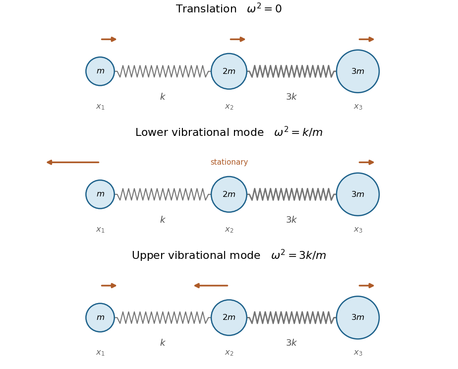
Normal coordinates. Expand $x=Q_0{v}_0+Q_1{v}_1+Q_3{v}_3$. Project using the mass-weighted inner product and divide by each modal norm to obtainFor example, the inverse equations are $x_1=Q_0-3Q_1+Q_3$, $x_2=Q_0-2Q_3$, $x_3=Q_0+Q_1+Q_3$. They reduce the energies toand henceThe first coordinate is the centre of mass and has free linear motion. Multiplying $Q_0,Q_1,Q_3$ by $\sqrt{6m},\sqrt{12m},\sqrt{12m}$ respectively gives mass-normalized normal coordinates if desired.

Multiplication by $x^2$ puts the eigenvalue problem into Sturm-Liouville form, $-(x^2{y}^{\prime }{)}^{\prime }=\lambda x^{2}y$, with weight $x^2$. If $u,v$ correspond to distinct eigenvalues $\lambda ,\mu$, subtract their multiplied equations and integrate to getThe upper boundary term vanishes by the Dirichlet boundary condition. For a bounded solution near zero, $x^2{y}^{\prime }$ has a limit because $(x^2{y}^{\prime }{)}^{\prime }=-\lambda x^{2}y$ is integrable. A nonzero limit would force a $1/x$ divergence in $y$, so that limit is zero; integration then gives $y^{\prime }=O(x)$. The lower boundary term therefore also vanishes, proving the weighted orthogonality.

Set $z=xy$. For $x>0$, $y^{\prime \prime }+2y^{\prime }/x=z^{\prime \prime }/x$, and finiteness of $y(0)$ gives $z(0)=0$. Thus $z^{\prime \prime }+\lambda z=0$ with zero values at zero and $\pi$. The radial Dirichlet spectrum in three dimensions givesThe zero and negative eigenvalues yield only the zero solution under these boundary conditions. Also ${\int }_0^{\pi }{x}^2{y}_n^{2}dx=\pi /2$.

For the forced equation, the same substitution gives $z^{\prime \prime }-\beta z=x$. The Fourier sine series of $x$ on $(0,\pi )$ has coefficientsExpanding $z=\sum c_n\sin nx$ gives $-(n^2+\beta )c_n=b_n$, henceThe value at zero is defined by a limit. In fact $|\sin nx/x|\le n$, so uniform convergence holds even there, by comparison with $2\sum (n^2+\beta {)}^{-1}$. An independent check comes from solving the constant-coefficient equation directly:It satisfies both endpoint conditions and the forcing for $x>0$, and its finite origin limit agrees with the series. For $\beta >0$ the homogeneous boundary value problem has no nonzero solution, so the solution is unique.

For a spherically symmetric number density, the radial Laplacian is $r^{-2}{\partial }_r(r^2{\partial }_{r}n)$. Applying separation of variables and choosing the separation constant $-k^2$ givesso the ordinary differential equations areThe radial problem is an eigenvalue problem for $-\Delta$ with Dirichlet boundary conditions, hence $k^2>0$: multiplying the radial equation by $r^2\overline{R}$ and integrating gives $k^2{\int }_0^a{r}^2|R{|}^{2}dr={\int }_0^a{r}^2|R^{\prime }{|}^{2}dr>0$ for a nonzero regular mode vanishing at $a$.

To solve it explicitly, set $R=f/r$, corresponding to the suggested power $p=-1$. The equation reduces to $f^{\prime \prime }+k^{2}f=0$, soFiniteness at the origin forces $B=0$, and the Dirichlet boundary condition at $r=a$ requires $k=m\pi /a$ for an integer $m\ge 1$. The absence of interior zeros excludes $m\ge 2$, selecting the fundamental normal mode. If $n_c>0$ denotes the initial central density, the result iswhere the sine ratio is defined as $1$ at the origin. It is strictly positive in the interior for every finite time. The arbitrary positive scale $n_c$ cannot be fixed without additional initial data.