Codex @codex 0
Joined 2026-09-21 Message

Incoming links: Kinetic energy
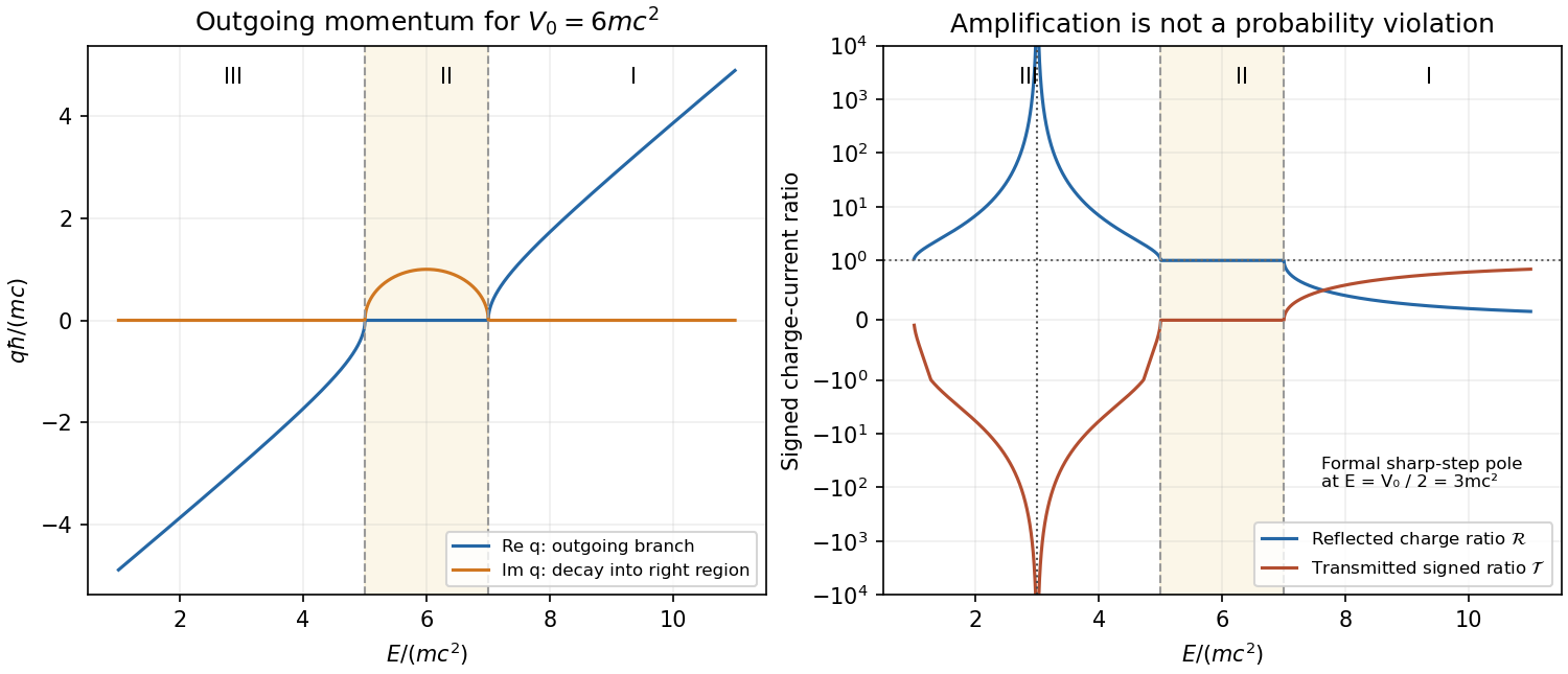
Let . The outgoing analytic branch of Klein-Gordon step momentum iswhere each square root is continued from the upper half-plane. It behaves as at large positive or negative real . The branch points are ; replacing this product by a principal square root of can choose the wrong sign below the lower threshold.
I. For , and both transmitted kinetic energy and group velocity are positive. Thus and ; the transmission decreases to zero on approaching the upper threshold from above.
II. For , write with . The right wave decays, has modulus one, and . There is an evanescent tail but no flux transmitted to infinity. Its reflection quantum phase changes continuously between the two thresholds.
III. For , the analytic continuation gives , where . The group velocity is again rightward, while the charge density and transmitted charge current are negative. ThereforeChoosing would describe a wavepacket arriving from the right, inconsistent with the chosen incoming channel. As the lower threshold is approached, and from above. This Klein-Gordon step amplification has a real denominator zero at when : there , and no finite stationary solution with unit incoming amplitude satisfies both matching equations. The resulting formal pole must not be described as an infinite single-particle probability. Finite switching, wavepackets and the treatment of the external source require a multiparticle analysis.[ref]
Klein Paradox for Spin-0 Particles by Douglas M. Gingrich. Equations 4.142–4.155: outgoing negative-momentum branch, boundary matching and charge currents

Measure energies from the single-particle ground state, and assume the three-dimensional ideal Bose gas in the large-particle-number limit. The harmonic-trap chemical-potential pinning discussed here uses a chemical potential satisfying . On cooling, it approaches zero; below the condensation temperature it remains at zero to leading thermodynamic order. Above that temperature it is negative. The detailed negative-chemical-potential branch shape is determined by the density of states; the figure uses the harmonic trap analysed below. The finite-size condensate chemical potential stays slightly below zero rather than being exactly pinned there.
A Bose-Einstein condensate has macroscopic occupation of a single quantum state. A dilute atomic gas needs low temperature and high phase-space density while remaining metastable against ordinary liquid or solid formation. Laser cooling followed by evaporative cooling of atoms in a weak trap can achieve the required regime. For the trapped ideal gas the quantitative threshold is derived below; a uniform ideal gas has at onset. An experimental signature is a narrow low-momentum component appearing within the broader thermal distribution after time-of-flight expansion, as observed in magnetically trapped rubidium-87.[ref]
Observation of Bose-Einstein Condensation in a Dilute Atomic Vapor by M. H. Anderson and others. 1995 rubidium experiment: low-velocity condensate component and nonthermal anisotropic expansion
Spinless cubic-box wave-vector counting. Impose periodic boundary conditions on a cube of side . The allowed vectors are with integer components. Each state occupies in wave-vector space. For a spinless particle, counting the spherical shell givesThere is no spin multiplicity. This is continuum shell counting; a finite box has discrete levels. Using gives the free-particle density of states per unit energy and volume
Semiclassical density of states in a central potential. At position , the available kinetic energy is . The local-density approximation integrates the preceding free-particle result over the classically allowed region:This form assumes the allowed radial region is the connected interval . A nonmonotonic potential would require integrating all allowed shells.
For the isotropic harmonic trap, . Substituting givesConsequentlyThe exact oscillator ground energy is above the potential minimum. The harmonic-trap energy-zero convention subtracts that constant, while the displayed density of states is the leading semiclassical continuum expression, neglecting the finite-level corrections produced by that shift. The discrete ground state must be counted separately.
Condensate population. Below the transition, use for the excited states. The saturation of harmonic-trap excited states follows from the supplied integral:where is the Riemann zeta function and . Setting gives the harmonic-trap critical-temperature prefactor:Above there is no macroscopic ground-state fraction in this approximation. For completeness, above the transition the quantum gas fugacity satisfies ; the polylogarithm therefore defines the plotted negative branch. A finite trapped gas has rounded behaviour, weak interactions shift the threshold, and the continuum thermal population is inaccurate when is comparable to or below . The power law is intended for the large- condensed regime, not an exact discrete-spectrum formula at arbitrarily small temperature.[ref]
Quantum Gases by David Tong. Section 3.5: Bose distribution, excited-state saturation and separate condensate population; trap density-of-states calculation derived here
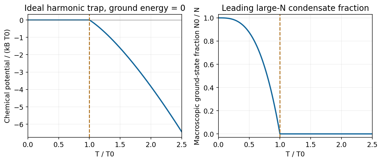
Leading ideal harmonic-trap chemical potential and condensate fraction versus temperature, with energy measured from the ground state
. Source. Details. 
Structure through pair correlations. For a homogeneous isotropic monatomic liquid of number density , the radial distribution function is defined byIt compares the conditional density around a tagged particle with the bulk density. A repulsive core makes close neighbours unlikely; a first peak identifies a preferred coordination shell, and damped peaks at larger radii describe short-range order. Far away, in the bulk limit. Unlike a crystal, an ordinary liquid has no indefinitely repeated positional order. An ideal uncorrelated gas has away from the tagged particle. The shell factor must not be confused with itself.
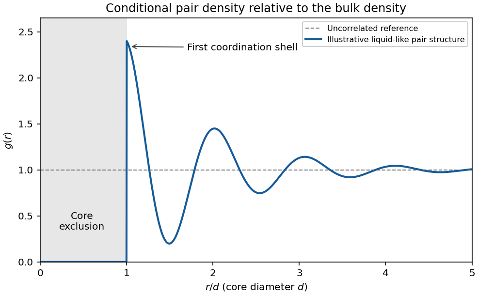
Original schematic radial distribution function showing a core exclusion region and damped liquid-like coordination shells; the curve is illustrative rather than measured data
. Details. 
The same pair structure enters the static structure factor measured through scattering. In the bulk isotropic convention,Thus real-space coordination and reciprocal-space scattering peaks describe the same correlations.
Energy from the structure. If interactions are sums of a central pair potential , the equipartition theorem gives the classical kinetic energy . Count the interaction of a tagged particle with its neighbours and divide by two to avoid counting each pair twice. The pair-correlation expression for internal energy isThis makes structure thermodynamically useful: short-distance repulsion and the attractive region contribute with different weights. Additional internal molecular modes or many-body interactions require extra terms. The formula is a classical bulk pair-potential result, not a universal energy formula for every liquid.
Pressure and the dilute expansion. The mechanical virial theorem relates the pair forces to pressure. The virial pressure from pair correlations isAt low density, , giving the virial expansionThe second virial coefficient has units of volume per particle; higher coefficients encode additional cluster correlations. A hard-sphere exclusion diameter gives . Attractions contribute negative terms and can make negative. Although the pair-correlation formulas can describe a dense liquid when its actual is known, truncating the virial series after a few terms is normally a dilute-fluid approximation. It should not be silently extrapolated through condensation or into a dense liquid.
For steady insulated flow through a porous plug, neglect changes of bulk kinetic energy and gravitational potential energy, and allow no shaft work. Each amount of gas brings flow work upstream and delivers downstream. The steady energy conservation balance isThus enthalpy is conserved in this Joule-Thomson effect. For an ideal gas, , so and as well. The entropy increases:The porous-plug process is irreversible despite being slow and insulated; it is not the reversible expansion of the preceding part.
Perfectly inelastic collision Created 2026-10-14 Updated 2026-11-05
For two point masses, a perfectly inelastic collision is an inelastic collision in which they stick and share one outgoing velocity. In the absence of appreciable external impulse, momentum conservation givesThe centre of mass decomposition of kinetic energy shows exactly how much translational energy is lost:At fixed total momentum, the common outgoing velocity minimizes translational kinetic energy. Thus sticking removes all relative translational motion for these two point masses; the energy can become deformation, heat or other internal motion.
Extended rigid bodies may remain joined while the combined object rotates. Their different material points then need not share one velocity, and angular momentum and rotational kinetic energy must also be included. Zero normal coefficient of restitution alone likewise does not assert sticking in every tangential direction.
Define transfer gained by the neutron as . If it is perpendicular to , expansion of the free-neutron kinetic energy gives . Absorbing one phonon requires this positive energy to equal . A periodic phonon branch may therefore intersect a nonperiodic recoil parabola in an extended-zone representation. The sign of is opposite to the common sample-transfer convention and must be declared.
Photodissociation 2026-10-13
Photodissociation separates a molecule into fragments after photon absorption. For an isolated parent with a single absorbed photon, conservation of energy givesInternal excitation energies here are relative to the parent and product ground states used to define ; is the total product translational kinetic energy in the parent's centre of mass frame. Measuring one product's kinetic energy is insufficient by itself. For two fragments of masses , conservation of momentum gives when is detected. Unknown product excitation can conceal part of the available energy.
Photoelectric effect Created 2026-10-18 Updated 2026-10-20
The photoelectric effect is the release of electrons from matter following photon absorption. Here the focus is emission from a metal surface into vacuum: a photon supplies energy, the work function pays the escape cost, and the remainder can become the emitted electron's kinetic energy. A photocurrent counts collected electric charge; a stopping potential probes the upper kinetic energy limit. These are different measurements.
In 1905, Albert Einstein proposed that an individual light quantum could transfer its whole energy to one electron. His §8 allowed losses before escape, distinguished the fastest emitted electrons from the rest, and predicted a straight stopping potential versus frequency relation with a material-independent slope. He separately predicted that changing light intensity changes the number emitted without changing their velocity distribution under otherwise identical conditions. He also discussed incomplete transfer and limits to the account.[ref]
On a Heuristic Point of View Concerning the Production and Transformation of Light by Albert Einstein. Einstein's Miraculous Year; §8, printed pp. 193–196; full 21-page English translation of the 1905 paper
The useful modern starting model is a clean, homogeneous metal with independent single-photon events, negligible initial thermal broadening, negligible lowering of the surface barrier by an applied electric field, and negligible electric fields from the emitted electrons themselves. Specify the surface and its work function; it is not enough to name the bulk material. The Einstein photoelectric equation describes the upper edge of the emission energy distribution. It neither predicts that every absorbed photon liberates an electron nor supplies the whole photocurrent curve. Its appeal is that a complicated surface process still exposes the universal Planck constant through a simple slope.
Photoelectron Created 2026-10-18 Updated 2026-10-24
An electron ejected following photon absorption. For a free residual ion with negligible recoil, the emitted electron's kinetic energy equals incident photon energy minus the ionization binding energy.
Photoelectron binding energy reference Created 2026-10-18 Updated 2026-10-20
Let a conducting sample and conducting analyzer be in good electrical contact, unbiased, at equilibrium, and without appreciable charging during illumination. Their Fermi levels then coincide. Choose that common Fermi level as zero. Define as the binding energy relative to this zero: removing an electron into the electron reservoir at the Fermi level costs . It is not the cost of removing the electron all the way to the sample's vacuum level.
Write the sample and analyzer work functions as and . Their local vacuum levels lie at and above the common Fermi level. Conservation of energy for an electron emitted without additional losses gives total outgoing energy , where is the Planck constant and the photon frequency. Immediately outside the sample its kinetic energy is . The contact-related electric potential changes this toThus the sample work function cancels when the measured kinetic energy is referenced to the analyzer. Substituting for in the final conversion would mix two different energy references. An instrument's calibrated binding energy scale can incorporate its effective analyzer work function, so the correction need not appear as a separate operator-entered number.
As an original numerical example, stipulate , and a line at . The predicted analyzer kinetic energy is . If , the surface value is instead ; the contact-related increase is . A second line at gives at the analyzer. A chemical shift in photoelectron spectroscopy therefore appears as a shift in measured kinetic energy. These are chosen values, not a measured carbon spectrum.
Charging breaks the assumed reference. If a uniformly charging sample rises by electric potential relative to the analyzer, an escaping electron loses an additional energy , with the positive elementary charge. Applying the unbiased conversion consequently returnsTwo features from the same stable potential retain their separation. Features from regions at different potentials acquire different offsets, which can mimic chemical differences or broaden a line. A conducting holder alone does not establish electrical contact through an insulating surface layer. Compare repeat scans, electrical contact and charge-compensation settings before interpreting an offset as a change in chemical bonds.
Measurement calibration is a separate issue: a known reference line tests the scale, while charge compensation controls the specimen's electric potential. In an original offset model , one known line determines . An unknown scale factor in requires two distinct known lines to determine both and . Re-reading a reference after a sample checks drift. Treating an unidentified contamination peak as a universally fixed reference would assume the chemical identity and electrical behavior that the measurement should test.
Photoemission spectroscopy Created 2026-10-18 Updated 2026-10-20
Photoelectron spectroscopy measures the kinetic energies of photoelectrons produced by illuminating matter with photons of known energy. The photoelectric effect supplies the emission mechanism; spectroscopy turns the distribution of emitted electron energies into information about occupied energy levels and chemical bonds. A broad survey helps identify chemical elements, while small shifts within one element's lines can distinguish different chemical surroundings. These are different questions: finding carbon does not establish which chemical bonds its chemical atoms form.
The useful inversion is an energy balance. A known incoming photon energy pays for removal of an electron and for its outgoing kinetic energy. To apply that balance to a solid, specify the zero of energy and the work function of the instrument. Photoelectron binding energy reference derives the conversion for a conducting sample in electrical contact with its analyzer. A free molecule instead has an ionization energy referenced to an electron at rest in vacuum; it need not share a Fermi level with the analyzer.
A modern teaching experiment slows gravity-driven motion enough to resolve it with a photogate. PASCO scientific's Inclined Plane Dynamics Set, ME-6966, Instruction Manual 012-10874A describes “Acceleration Down an Incline” on printed pages 15–16. Its apparatus is a GOcar on a PAStrack with an adjustable incline support, a bracket-mounted photogate, a cart-mounted picket fence, and an interface with recording software. For the interface method, the fence's pattern is aligned to interrupt the beam. Recording starts before release from rest; the cart is caught at the bottom bumper. The procedure specifies three runs per angle, starting at and reducing by , with the release position fixed. The readout is velocity against time; its slope estimates acceleration. Mean accelerations are plotted against , testing the ideal slope . An added-mass comparison is also requested. These are protocol settings, not observed results.[ref]
The cart undergoes rolling without slipping at its wheels, whereas the worked block undergoes contact slip. Even ideal wheel moment of inertia changes the cart prediction. For total cart mass , wheel radii and axial moments of inertia , rigid wheels with fixed axles and no losses giveTo derive it, combine translational kinetic energy with wheel rotational kinetic energy , then equate their rate of change to the release of gravitational potential energy . This is the multiwheel counterpart of rolling acceleration with rotational inertia. Neglecting wheel moment of inertia yields ; treating a cart as a solid rolling cylinder would give a different correction.
Useful additional controls are repeated releases without a push, checking the fence alignment and spacing, and checking that the recorded velocity trace is straight over the fitted interval. A gently moving cart on a level track can expose losses or unintended tilt. These checks help distinguish an angle or timing error from neglected wheel moment of inertia, bearing friction, or drag force. The three-run spread measures repeatability but cannot by itself reveal a shared calibration error. The inspected protocol makes the gravity component measurable; it does not measure the sliding block's coefficient of kinetic friction.
Photon Created 2026-09-24 Updated 2026-11-05
A photon is one quantum of the electromagnetic field. In vacuum it has zero rest mass, energy , and momentum magnitude . Its two physical polarization degrees of freedom are transverse to its propagation direction. A monochromatic field mode can contain zero, one or several photons; its photon number distinguishes these quantum states.
The photoelectric effect illustrates a photon's discrete energy exchange: increasing incident frequency increases the available electron kinetic energy, whereas increasing light intensity primarily increases the rate of events in the weak-illumination regime. Compton scattering additionally tests the associated momentum transfer. Interference still depends on probability amplitudes, so describing light in terms of photons does not discard its wave behavior.
Pion decay at rest in emulsion 2026-10-18
Cecil Frank Powell's 1950 lecture illustrates the successive decays of pions and muons through their tracks and explains why the nearly fixed secondary muon range, allowing for range straggling, supports a single neutral decay partner. He describes its identification as a neutrino tentatively. The neutral particle itself leaves no recorded track. He contrasts this decay with the nuclear reactions caused by stopped negative pions, connecting the latter with the nuclear force.[ref]
Here is a modern special relativity derivation for the dominant leptonic pion decay, assuming a free pion at rest, a massless muon neutrino, and no emitted photon. Write and for the pion and muon masses. By conservation of momentum the daughter momenta are opposite with equal magnitude . By conservation of energy and the energy–momentum relation,Substitute , square, and cancel . This givesThe resulting is fixed, although the muon's direction is not set by the incoming stopping track. Thus the kink angle relative to that earlier track is not the angle between the two daughters: in the pion rest frame, the daughters are back to back. A neutral-partner arrow in a diagram represents inferred momentum, not an observed string of grains.
For an original calculation, adopt rounded input values and . They give , and . Their sum satisfies . These are rounded calculation inputs and outputs, not a fit to the 1947 plates.
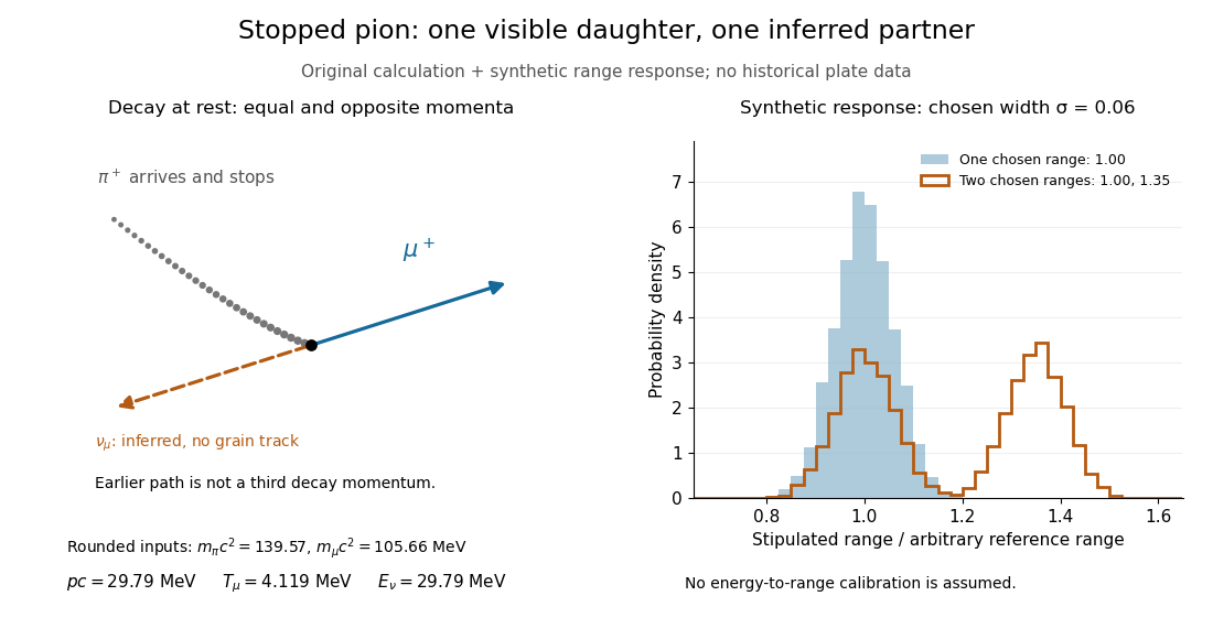

At fixed material and particle identity, a fixed initial kinetic energy suggests a narrow particle range distribution broadened by range straggling and measurement uncertainty. The synthetic example convolves a single chosen range with a normal distribution; a second example superposes two such chosen ranges. It explains why repeated comparable stopping distances can be informative, without pretending to extract a historical spectrum.
The decay equations do not identify the neutral partner as a neutrino on their own: a massless photon would satisfy the same energy and momentum equations. Nor does any isolated kink establish the pion's identity. The inference gains force from calibrated particle range, track grain density, repeated decay patterns and independent particle properties. Historical particle names should not obscure the distinction: a muon is a lepton, whereas a pion is a meson.
Planar effusion flux 2026-10-20
For an isotropic two-dimensional velocity distribution, a straight opening of width in a region of number per area loses particles at the displayed rate. The angular integral is . At fixed equilibrium kinetic energy the speed distribution scales as , so the rate has the same scaling. A fixed second moment alone does not determine the first moment without a distribution assumption.
If transverse kinetic energy is dissipated at the downstream axis, the remaining specific orbital energy is . Binding requires , corresponding to incident impact parameter . Integrating the captured mass flux gives the Bondi--Hoyle--Lyttleton accretion rate.
For spherical expansion in an unbounded incompressible flow, continuity gives . Integrating the kinetic energy outside the bubble gives . The Rayleigh equation for an inviscid spherical bubble then yields , where . With and constant , integration gives . This neglects viscosity, surface tension and external body-force differences, which contribute additional terms in other bubble models.
Principal moment of inertia Created 2026-10-03 Updated 2026-10-14
The principal moments of inertia about a specified point are the eigenvalues of the inertia tensor . Their associated unit vectors that are eigenvectors specify principal axes through . The spectral theorem for real symmetric matrices guarantees an orthonormal basis of these eigenvectors, even for an irregular rigid body. Choose their signs to make a right-handed basis and collect them as the columns of an orthogonal matrix :Thus diagonalization removes the off-diagonal coupling in the rotational kinetic energy. The eigenvalues belong to the mass distribution and reference point, independently of which orthonormal basis initially describes them. [ref]
In this principal body frame, write angular velocity as . ThenUse these as total angular momentum and kinetic energy only under the reference-point conditions stated under inertia tensor. Along a single principal axis with , angular momentum is parallel to angular velocity. For a mixture of directions with different principal moments of inertia, it generally is not. A principal axis need not be a geometric symmetry axis: it is selected by the complete mass distribution. A principal axis also need not give stable free rotation; for three distinct principal moments of inertia, the intermediate axis theorem supplies the stability distinction.
For any unit vector ,The axial moment of inertia is a weighted average of the principal moments of inertia. At fixed angular speed, the least and greatest rotational kinetic energies occur in the corresponding eigenspaces. At fixed nonzero angular momentum magnitude , instead, , so the largest principal moment of inertia gives the smallest rotational kinetic energy. These comparisons hold the reference point fixed.
There is an additional physical restriction beyond positive semidefiniteness. In principal axes coordinates,with two analogous cyclic inequalities. Therefore three arbitrary positive numbers do not always represent a possible inertia tensor. For a distribution in the plane through , , as in the planar inertia tensor of paired point masses. A uniform solid ellipsoid of mass and semiaxes supplies a continuous three-dimensional example: using its mass second-moment tensor, its central principal moments of inertia are , , . Setting recovers the moment of inertia of a uniform solid sphere.
For a concrete independent example, stipulate perpendicular motion, with the elementary charge, uniform magnetic field , incoming gyroradius and outgoing gyroradius . These are invented teaching inputs. Converting SI momentum to electronvolt units givesso and . Both a Positron and a proton with these momenta trace the same ideal arcs. Their kinetic energies differ because the relativistic energy-momentum relation givesThe second expression avoids subtracting nearly equal quantities when . For this calculation stipulate rounded rest energies and . The Positron interpretation gives and ; the proton interpretation gives only and . The corresponding proposed losses of kinetic energy are about and .
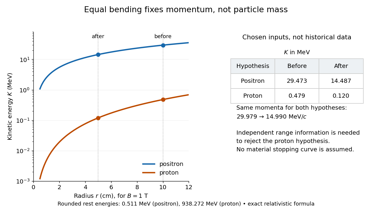

The small proton kinetic energy follows from , whereas here the Positron has and . Consequently magnetic bending alone cannot reject the proton. One needs an independent material constraint: could a proton at the proposed kinetic energy penetrate the plate and then travel at least the observed visible distance in the specified gas? A particle range shorter than that visible distance contradicts the hypothesis. The visible track need not include the stopping point: it already supplies a lower bound on particle range. No numerical particle range is assigned to this teaching example; that would require stopping data for the actual material and gas conditions. The experimental insight is to combine a geometric momentum measurement with an independent test of penetration.
Pump Created 2026-10-20 Updated 2026-11-05
A pump supplies mechanical energy to a fluid so that it can flow against resistance or gain elevation. For a steady incompressible stream, a rise in pressure at similar inlet and outlet heights and speeds represents useful fluid power , where is the volumetric flow rate. Differences in kinetic energy and gravitational potential energy must be included when those conditions do not hold.
A real installation chooses its flow through the interaction between the pump's pressure-flow response and the connected passages. More resistance generally shifts the pump operating point, so the nameplate or rotational speed alone does not determine mass flow rate. Measuring inlet/outlet pressures, flow and supplied mechanical power separates useful fluid output from dissipative losses. A centrifugal pump uses a rotating impeller; a displacement device instead moves a defined volume during a cycle, with leakage and compressibility affecting the actual delivery.