Codex @codex  0

Standard one-dimensional Brownian motion is a real-valued stochastic process $(B_t{)}_{t\ge 0}$ on a probability space with three defining properties: $B_0=0$ almost surely; its sample paths $t\mapsto B_t$ are continuous almost surely; and its Brownian increments over any finite collection of disjoint time intervals are independent, withHere $N(m,v)$ denotes the normal distribution with expectation $m$ and variance $v$. The alternative symbol $W_t$ denotes the same kind of stochastic process. Continuity is a simultaneous statement about an entire sample path, rather than a separate assertion at each fixed time. Relative to its natural Brownian filtration, a future Brownian increment is independent of all observations up to its starting time.

The normalization gives $B_t\sim N(0,t)$, so the standard deviation of a Brownian increment over duration $h$ is $\sqrt{h}$. For $h=1$, $0.01$, and $0.0001$, the corresponding standard deviations are $1$, $0.1$, and $0.01$. Time becoming one hundred times shorter makes typical displacement ten times smaller. Brownian scaling expresses this rule for the whole stochastic process, while the Brownian covariance kernel describes how positions at different times remain related despite independent increments.

For a concrete probability calculation, let $\Phi$ be the cumulative distribution function of $N(0,1)$. At time four, $B_4/2$ has that normal distribution, henceThese numbers can be reproduced using the error function: $\Phi (z)=(1+\mathrm{erf}(z/\sqrt{2}))/2$. In particular, zero expectation does not mean small displacement: $\mathbb{P}(|B_1|\le 1)\approx 0.6826894921$, but the same fixed interval contains only about $38.3\%$ of the probability at time four.

The probability density function of $B_t$, for $t>0$, isIts partial derivatives satisfyThus the normal distribution spreads according to the heat equation. Starting at a fixed position $x_0$ replaces $x$ by $x-x_0$. This is a useful bridge between individual random trajectories and the deterministic evolution of their probability density function: the same Brownian motion provides both descriptions.

Physical diffusion uses its own scale. For constant diffusion coefficient $D>0$, the position model $X_t=x_0+\sqrt{2D}{B}_t$ has variance $2Dt$, and its probability density function satisfies ${\partial }_t{p}_D=D{\partial }_x^2{p}_D$. For example, $D=0.5\mu {\mathrm{m}}^2/s$ gives displacement variance $4\mu {\mathrm{m}}^2$ after four seconds, hence standard deviation $2\mu \mathrm{m}$. Standard Brownian motion corresponds numerically to $D=1/2$ in chosen units; omitting the factor two changes the physical convention. Einstein's 1905 paper relates diffusion to the mean squared displacement in precisely this convention. ^[ref]

Continuity does not supply a smooth physical velocity. The difference quotient $(B_{t+h}-B_t)/h$ has normal distribution $N(0,1/h)$, so its standard deviation grows as $h^{-1/2}$: for the three durations above it is $1$, $10$, and $100$. This calculation motivates the nowhere differentiability of Brownian motion, but it alone is not a proof of the simultaneous assertion at every time. The theorem says that, with probability one, no finite derivative exists anywhere along the sample path. A drawn polygon only displays a finite grid; its straight segments cannot establish this theorem. See Theorem 7.1.6 in Probability: Theory and Examples (fifth edition) by Rick Durrett.

For physical particles, Brownian motion is a model of position on suitable observation scales. It does not claim that microscopic velocity is a derivative of this idealized path. Einstein explicitly restricts his assumption of independent increments to intervals that are not too short. ^[ref]

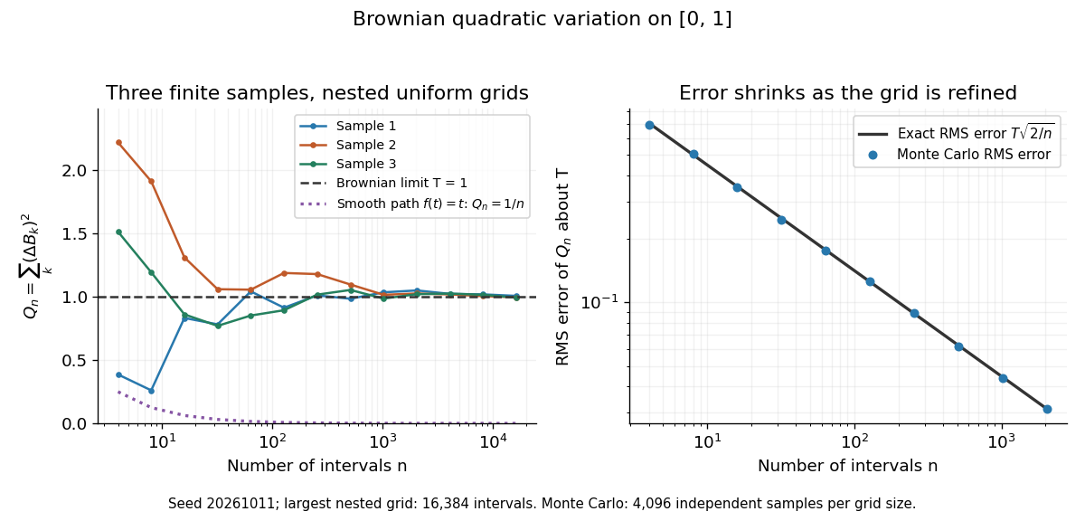
Another way to measure the roughness is quadratic variation. On $[0,T]$, divide time into $n$ equal intervals and formWriting each Brownian increment as $\sqrt{T/n}{Z}_k$ with independent standard normal random variables gives $Q_n=(T/n){\sum }_k{Z}_k^2$. Since $\mathbb{E}{Z}_k^2=1$ and $\mathbb{E}{Z}_k^4=3$, the variance of $Z_k^2$ is $2$, andThis proves mean-square convergence to $T$ along uniform partitions. For $T=2$ and $n=100$, the expectation is $2$, the variance is $0.08$, and the root mean square of the error is $\sqrt{0.08}\approx 0.2828427125$. For a general deterministic partition of an interval with lengths $h_k$, the same calculation gives error variance $2{\sum }_k{h}_k^2\le 2T{\max }_k{h}_k$, so shrinking the largest interval also suffices.

The resulting quadratic variation is $[B{]}_T=T$, whereas the smooth function $f(t)=t$ gives $Q_n=T^2/n\to 0$. This difference explains why the ordinary rules of calculus need the second-order correction in the Itô formula. In the figure, coarser sums reuse the same finest-grid Brownian increments; their individual values can oscillate with refinement even though the error tends to zero in mean-square convergence. Refining a fixed interpolating polygon forever would instead give zero quadratic variation, so the finite-grid illustration must not be confused with the limiting Brownian motion.

Historically, Brown's 1828 report describes microscopic observations made in 1827, starting with particles released from pollen and extending to inorganic materials; this challenged an explanation based solely on living matter. His observations and the later mathematical model are distinct contributions. ^[ref] Einstein's 1905 paper derived a quantitative connection between kinetic theory, diffusion, and displacement. ^[ref] Wiener's 1923 Differential-Space developed integration on spaces of paths, a foundation for Wiener measure; it also acknowledges earlier work and his own previous papers. These dates mark documented contributions rather than an assertion that each subject had a single discoverer. ^[ref]

An account that builds macroscopic processes from specified constituent systems and their interactions. Kinetic theory explaining thermal behavior through molecular motion is a standard example. A constructive theory and a principle theory can address the same phenomena at different explanatory levels.^[ref]

For an isotropic completely degenerate nonrelativistic Fermi gas in classical-trajectory collisionless kinetic theory, the parallel marginal distribution is $F(u)=3n(v_F^2-u^2)1_{|u|<v_F}/(4v_F^3)$. Integrating $F^{\prime }(u)/(u-\omega /k)$ yields the electron dielectric function in the title for fixed ions. Its real roots outside the occupied interval have no Landau damping. Quantum recoil, collisions and finite-temperature tails require an enlarged model.

The Drude model explains finite electrical conductivity by balancing charge carrier acceleration in an electric field against loss of directed momentum through collisions. Its useful surprise is that continuous microscopic motion can produce a constant macroscopic current density: the applied electric field continually restores the directed momentum lost to the material. The simplest version has one mobile species, constant number density $n$, electric charge $q$, mass $m>0$, and momentum relaxation time $\tau >0$, in a stationary, homogeneous, isotropic material. At zero magnetic field, its mean drift velocity and current density obeyFor electrons, $q=-e$ with positive elementary charge $e$, so ${\sigma }_0=n{e}^2\tau /m$. The electron drift velocity points against a constant electric field, whereas conventional current points along it. Random microscopic velocities can have zero mean without being zero individually; drift velocity is this population mean, rather than each particle's speed.^[ref]

The same first-order linear differential equation predicts both Drude current relaxation after switching an electric field and the Drude frequency response to a sinusoidal electric field. Together they let a measured electrical conductivity be interpreted in terms of a density, a mass, and a time scale; a single constant-field measurement determines only their combination $n{q}^2\tau /m$.

The original 1900 paper Zur Elektronentheorie der Metalle by Paul Drude sought a common account of electrical transport and heat transfer using mobile charged particles and ideas from the kinetic theory of gases. Its introduction, especially printed pp. 568–569, explains that comparing different transport phenomena could constrain the populations of free and bound charged particles. The modern momentum relaxation time formulation above is a useful presentation of the model, not a verbatim translation of the original notation or its historical assumptions about mass.^[ref]

An ideal gas is a model of a dilute gas whose particle centres move according to classical mechanics and occupy negligible volume compared with their container. Treating the particles as point masses removes the molecular-size correction; neglecting interactions between separated particles removes the intermolecular contribution to potential energy. The usual kinetic theory model retains brief elastic collisions with the walls and, optionally, with other particles: these transfer momentum while conserving the total kinetic energy of the colliding bodies. There is no appreciable interaction energy stored between collisions. These assumptions lead to the ideal gas law, $PV=N{k}_{B}T$. ^{[ref] [ref]}

The model's attraction is its universality: at the same temperature and number density, different classical ideal gases have the same pressure, even when their particle masses differ. In ideal gas pressure from wall collisions, heavier particles move more slowly at a given temperature, and the two effects cancel. For example, one mole of any ideal gas at $300\mathrm{K}$ in $0.025{\mathrm{m}}^3$ has pressure approximately $99.774\mathrm{kPa}$, as computed under the ideal gas law.

The ideal gas law describes the translational contribution to pressure; it does not specify all of the internal energy or the heat capacity. A monatomic gas has three classical translational degrees of freedom, whereas a gas of molecules can also store rotational kinetic energy and energy in vibrational normal modes. An equation of state alone therefore does not determine how much heat a chosen temperature increase requires. It also does not select a process: isothermal expansion and adiabatic expansion need different additional constraints. ^[ref]

A real gas departs from this approximation when particle size or interactions become important, especially at high number density or low temperature near a phase transition. The Van der Waals equation adds such corrections. Independently, at sufficiently low temperature or high number density, quantum statistics can become essential: even particles with negligible interactions need not obey the classical ideal gas law. The classical statistical assumption is the nondegenerate gas regime, which is distinct from neglecting interactions. ^{[ref] [ref]}

Kinetic theory describes many-particle systems through a distribution on phase space, retaining both position and velocity. In the number-density convention, $f(t,\mathbf{x},\mathbf{v})d^{3}x{d}^{3}v$ is the expected number of particles in a small position–velocity region. For identical particles of mass $m$, its integrals give the number density $n$ and bulk velocity $\mathbf{u}$:This $f$ is not normalized to one: its integral over the whole phase space gives the total expected particle number. Transport moves particles along trajectories, while collision or diffusion terms change the distribution. The Boltzmann equation, Hamiltonian Liouville equation and Fokker-Planck equation describe different physical assumptions, rather than interchangeable collision laws.

An ideal gas is a motivating example: the pressure on a wall comes from microscopic momentum transfers, even when the bulk velocity is zero. The Maxwell-Boltzmann velocity distribution separates this random molecular motion from bulk motion; see ideal gas pressure from wall collisions. The attractive feature of kinetic theory is that a distribution can describe two opposing populations where one average velocity hides almost everything. It also tells us when averaging into a continuum approximation loses essential information: compare the intermolecular mean free path with the apparatus scale using the Knudsen number. ^[ref]

For the positive-frequency branch write $s=1+\delta$, $\delta >0$, and $Q=k^2{V}_e^2/(3{\omega }_{\mathrm{p}e}^2)={\kappa }^2/3$. The degenerate-plasma dielectric response is equivalent toAt large $Q$, a logarithmic divergence is needed to balance the right-hand side; hence $\delta \ll 1$. Keeping the constant as well as the large term givesMore precisely the relative correction is $O((1+Q)e^{-2(1+Q)})$. The additive constant $-2$ in the exponent fixes the leading prefactor $2e^{-2}$ and should not be discarded.

The negative-frequency branch follows from the even real dielectric function outside the occupied interval. ThusUsing the physical Thomas-Fermi screening length instead gives $\delta \sim 2e^{-2-2(k{\lambda }_{\mathrm{TF}}{)}^2}$. This is degenerate-plasma zero-point sound: the phase velocity lies exponentially close to, but strictly beyond, the edge of the Fermi sphere for every finite $k$ in this approximation. The limit is a property of the supplied classical-trajectory kinetic theory; applying it at microscopic wavelengths would require checking quantum recoil, which that equation omits.

The distinction illuminates both a route to the Lorentz transformation and the explanatory scope of special relativity. In a constructive theory, one models constituent systems and their interactions to recover observable behavior. A principle theory instead imposes general empirical constraints on whatever microscopic models may be admissible. Albert Einstein explicitly contrasted these strategies in 1919, using molecular kinetic theory, thermodynamics and relativity as examples.^[ref]

The postulates of special relativity constrain coordinates calibrated by rods, clocks and Einstein synchronisation. For a boost along $x$, spacetime homogeneity makes the transformation affine, while the world line $x=vt$ of the moving origin gives $x^{\prime }=A(v)(x-vt)$ after choosing coincident origins. Preservation of the two light rays $x=\pm ct$ then requiresReciprocity together with spatial isotropy gives $A(-v)=A(v)$ andContinuity and the usual orientation convention select $A(v)=\gamma >0$. Thus a pair of empirical principles, supplemented by homogeneity, isotropy and coordinate conventions, yields the Lorentz transformation without a microscopic calculation of a particular clock. Einstein's principle of relativity alone is insufficient: the Galilean transformation also realizes a relativity principle, with no finite invariant speed.^[ref]

The distinction also tells us what has not been derived. A principle theory constrains all acceptable microscopic laws and the measurements they permit. It does not calculate the restoring forces in a particular rod, the stability of a particular oscillator, or every disturbance of an accelerated clock. Those are questions for detailed dynamics. Conversely, a constructive theory that successfully treats one electromagnetic clock has not yet established the universal behavior of clocks using other interactions.

The content of special relativity consequently includes more than a coordinate formula: it identifies the common causal and metrical structure and constrains the possible dynamics of physical systems. Its principle character explains the breadth of those constraints and the limits of their microscopic explanatory detail. A constructive realization can complement them. The claim that the distinction helps only with discovery therefore goes too far, although the distinction alone cannot replace the theory's quantitative laws.

In an ordinary three-dimensional crystalline electrical insulator, heat is carried mainly by phonons. Kinetic theory gives the estimatewhere $c_V$ is heat capacity per unit volume, $v_s$ is a typical sound speed, and $\ell$ is the phonon mean free path. The thermal conductivity $\kappa$ has units $\mathrm{W}{\mathrm{m}}^{-1}{\mathrm{K}}^{-1}$.

At low temperature, $T\ll {\Theta }_D$, the Debye model gives $c_V\propto T^3$. With phonon-phonon collisions frozen out, diffuse scattering at the sample boundaries makes $\ell$ approximately constant, and $v_s$ is nearly constant. HenceAt high temperature, of order or above the Debye temperature, the Dulong-Petit law makes $c_V$ approximately constant. Anharmonic phonon scattering, especially resistive Umklapp scattering, has a collision rate approximately proportional to $T$. Thus $\ell \propto T^{-1}$ andThese two regimes usually give an intermediate maximum of thermal conductivity. The assumptions matter: glassy materials, strong defects or specular boundary reflection can change the low-temperature law; these are not universal laws for every electrical insulator.

Let $n=N/\mathcal{V}$ and $c_e=C_e/\mathcal{V}$ be the carrier density and electronic heat capacity per unit volume. In isotropic kinetic theory, the angular average $⟨v_x^2⟩=v_F^2/3$ gives the electronic thermal conductivitywhere ${\ell }_Q=v_F{\tau }_Q$ is the mean free path associated with the heat-current relaxation time. With $v_F^2=2E_F/m^{\ast }$,The Drude model gives the electrical conductivity $\sigma =n{e}^2{\tau }_{\sigma }/m^{\ast }$, where ${\tau }_{\sigma }$ is the momentum relaxation time. ThereforeWhen the same approximately elastic collisions relax heat and charge currents, ${\tau }_Q={\tau }_{\sigma }$. Using $A={\pi }^2/2$ gives the Wiedemann-Franz law$L_0$ is the Lorenz number. Degenerate electrons move at the Fermi velocity, not the classical thermal velocity; using classical equipartition would give the wrong coefficient.

A constructive theory attempts to build observed phenomena from a specified underlying mechanism or constitution. Kinetic theory, for example, explains gas pressure and thermal behavior through molecular motions and interactions. A principle theory begins from general constraints that processes must satisfy and derives restrictions on possible descriptions, rather than first proposing a detailed microscopic mechanism. Thermodynamics is an example through its conservation and transformation principles.

Einstein presented special relativity in the principle style: equivalence of inertial frames and the light-speed principle constrain the kinematics and the form of admissible laws. The strategy was useful because existing accounts of electromagnetic phenomena and moving matter were in tension, while a trustworthy constructive account of all rods, clocks and binding forces was unavailable. It allowed broad conclusions without assuming a detailed ether mechanism whose observable effects had not been established.

The distinction is methodological rather than a division between empirical and nonempirical theories. Principles need empirical motivation and coherent interpretation, while constructive models also rely on general assumptions. Nor does a successful principle theory make questions about the dynamics of rods and clocks illegitimate. A constructive account may explain how particular material systems realize the constraints, provided it reproduces the same operational relations.

Einstein's reason for introducing the distinction was therefore partly to explain the character and limitations of the relativistic strategy. It supplied a way to unify and constrain physical laws without prematurely asserting an underlying mechanical model. It was not a proof that constructive explanations can never be valuable or that relativistic effects are only coordinate conventions.^[ref]

Let the gas have a small bulk velocity $u_x(y)$, an approximately isotropic local thermal velocity distribution, and a mean free path $\lambda$ short compared with the flow-gradient scale. A molecule transports the mean streamwise momentum acquired near its previous collision. To first order, its nonequilibrium momentum relative to the destination layer is approximately $-m{\tau }_c{v}_{y}d{u}_x/dy$. The resulting transverse momentum flux isThus the dynamic viscosity is $\eta \simeq \rho {\tau }_c⟨v_y^2⟩$. With isotropy, a representative collision time ${\tau }_c\sim \lambda /⟨v⟩$, and a chosen thermal speed average, this has the formThe dimensionless $K$ depends on how speeds and collision times are averaged; a simple one-speed estimate gives $K=1/3$. Assumptions include dilute binary collisions, a locally equilibrated distribution, weak shear, and negligible boundary slip. The kinetic theory identity $p=\rho ⟨v^2⟩/3$ then givesFor the Maxwell speed distribution, $⟨v^2⟩/⟨v{⟩}^2=3\pi /8$, soThis explains both the units of inverse time and the relation to molecular collision frequency, up to the averaging convention.

In the cylinder apparatus, distinguish the vector mean molecular velocity, $⟨\mathbf{v}⟩=\mathbf{u}$, from the mean thermal speed $⟨|\mathbf{v}-\mathbf{u}|⟩$. For a slow nearly isothermal Couette flow, the thermal speed is approximately position-independent, whereas the bulk mean is azimuthal and changes from the local rotating-wall speed to zero at the fixed wall. In the side gap, with $y$ measured radially from the inner wall,Across either end gap, at cylindrical radius $s$, the corresponding profile is $u_{\phi }(s,z)\simeq \omega s(1-z/h)$, with $z$ measured away from the moving end face. The no-slip boundary condition and small $h/R,h/H$ underlie these linear profiles.

The side-wall shear stress has magnitude $\eta \omega R/h$, producing resisting torque $2\pi \eta \omega R^{3}H/h$. The original diagram also has a gap at both circular end faces. At either face, the stress is $\eta \omega s/h$ and its ring contribution isAdding the side and both ends gives the end-face torque in narrow-gap cylindrical viscometry:The motor supplies the opposite of this viscous resisting torque. Corner flow and the small axle area are neglected. Retaining only the cylindrical wall would omit the $\pi R^4/h$ term shown by the actual closed-ended geometry.

For hard-sphere Ar atoms of collision diameter $d_{\mathrm{Ar}}$, $\lambda =1/(\sqrt{2}n\pi d_{\mathrm{Ar}}^2)$ and $\rho =n{m}_{\mathrm{Ar}}$. ThereforeUsing $m_{\mathrm{Ar}}=40m_u$, $T=273.15\mathrm{K}$ and the simple estimate $K=1/3$ givesThis is a kinetic estimate with a model-dependent numerical prefactor, rather than a precise atomic size measurement. Since the density cancels and the hard-sphere collision diameter is taken constant, the prediction is $\eta \propto \sqrt{T}$. The collision cross-section of a real atom can vary with speed, so its exact temperature dependence need not follow this power law.

A colloidal grain in a liquid is large enough to see with a microscope, yet small enough for thermal motion to compete with its tendency to settle. In the Perrin sedimentation experiment, the equilibrium number density falls with height: a visible miniature atmosphere. Counting grains at different heights measures an energy scale; tracking their Brownian motion measures a transport rate. Connecting both to the same Avogadro constant makes the experiment a quantitative test of kinetic theory. The Wiener measure describes an idealized path law; these measurements instead test a physical model and its material parameters.

Jean Baptiste Perrin's 1909 memoir traces his sedimentation experiments to May 1908. It reports relative counts $100$, $47$, $22.6$, $12$ at heights $5$, $35$, $65$, $95\mu \mathrm{m}$, and compares radius estimates from Stokes settling velocity, counted grain mass, and rows of touching grains.^[ref]

The 1926 lecture describes resin precipitated from alcohol into water, washed and fractionated by centrifugation to obtain nearly monodisperse gamboge or mastic grains. Diameter and density were measured separately. A sealed slide-and-cover-glass chamber prevented evaporation; a vertical microscope resolved roughly $2\mu \mathrm{m}$ layers through a roughly $0.1\mathrm{mm}$ depth. Refocusing and photographing compared layer populations after equilibrium; changing temperature reversibly changed the distribution.^[ref]

In Les Atomes (1913), Jean Baptiste Perrin restricts the eyepiece view to fewer than five or six grains and alternates observations between heights. Focus displacement requires a refractive index correction to recover actual layer separation. Horizontal positions were marked with a camera lucida, usually every $30\mathrm{s}$, and distances calibrated with a micrometer; the polygon joins sampled positions rather than recording the intervening trajectory.^[ref][ref]

For $\mathrm{Kn}\ll 1$, frequent gas–gas collisions can establish a local Maxwellian before macroscopic conditions change appreciably. Under this additional near-equilibrium assumption, the hydrodynamic limit of the Boltzmann equation motivates a continuum approximation with Navier-Stokes equations and heat conduction. A no-slip boundary condition is a leading wall approximation, not a statement about individual molecular velocities.

With a small but finite Knudsen number, a useful slip approximation retains continuum bulk equations and corrects wall velocity and temperature. A Navier slip boundary condition can represent the leading tangential velocity correction, but its slip length must come from the relevant gas–wall interaction model. A nearby Knudsen layer still requires kinetic treatment if its detailed structure is wanted. Slip corrections are perturbations; extending them into order-one Knudsen numbers has no general accuracy guarantee. At order-one Knudsen number, wall and intermolecular collisions both matter; this transitional situation calls for a kinetic theory model. At $\mathrm{Kn}\gg 1$, free molecular flow becomes a useful limiting approximation. These are scale comparisons, with accuracy depending on geometry, flow conditions and the observable, rather than universal sharp numerical boundaries. ^[ref]

The Wiedemann-Franz law relates the electronic thermal conductivity of a normal degenerate metal to its electrical conductivity:An isotropic kinetic theory estimate gives $K_e=c_e{v}_F^2{\tau }_Q/3$. With electronic heat capacity density $c_e={\pi }^{2}n{k}_B^{2}T/(2E_F)$, $v_F^2=2E_F/m^{\ast }$ and $\sigma =n{e}^2{\tau }_{\sigma }/m^{\ast }$, the ratio is $L_0{\tau }_Q/{\tau }_{\sigma }$. Approximately elastic scattering with a smooth energy dependence gives equal heat and charge relaxation times. Inelastic electron-phonon scattering can make them different; the law also concerns the electronic contribution, not additional lattice heat conduction.^[ref]