The original cover identifies 15 June 2018 despite the bundle filename. All six questions are treated. The missing Hall-voltage graph prevents the numerical calibration and field-specific assignments in Question 6; affected solutions contain explicit TODOs. Readings of the surviving graphs are approximate.
A phonon is one quantum of a normal vibrational mode of a crystal. In the harmonic approximation, each mode with wavevector , branch index and angular frequency is an oscillator with energies . A phonon changes the occupation by one; it is not a particular atom moving through the solid.
For a three-dimensional primitive cell containing atoms there are branches. Three acoustic branches approach zero frequency as : at zero wavevector they represent rigid translations, with all basis atoms displaced together. Their small-wavevector frequencies usually grow linearly with wavevector. The remaining optical branches have internal relative motion of basis atoms and generally nonzero zone-centre frequencies. The names reflect their coupling to radiation in suitable polar crystals, not a rule that every optical mode must be infrared active. Acoustic and optical branches can each have longitudinal or transverse polarizations.
Each atom supplies three displacement coordinates. Translational invariance gives three acoustic branches for either structure, leavingThese count branches at a general wavevector; a doubly degenerate pair still counts as two modes. The stated atom counts refer to primitive cells, so no additional centring factor is needed.
To obtain a crystal's point group, discard the translation parts of its space-group operations. A screw becomes a rotation and a glide becomes a mirror. Thus the tetragonal group's , and operations giveFor the orthorhombic structure the three perpendicular twofold/glide or screw/mirror directions giveThe primitive Bravais lattice symbol does not itself add a point operation; the fractional translations matter for the space group but disappear from this point-group reduction.
At the zone centre, the dynamical matrix commutes with the point-group representation on displacements. An irreducible representation of dimension two enforces a doublet; distinct one-dimensional representations need not have equal frequencies. The tetragonal point group has two-dimensional and representations, so optical modes transforming that way are doubly degenerate at the centre. Atomic positions and the displacement representation would be needed to assign every optical branch to a particular representation; the point-group label alone is not a complete mode decomposition.
For propagation along the tetragonal fourfold axis, the two transverse acoustic polarizations transform together and have equal sound speeds and frequencies. For example , whereas the longitudinal speed is independent. An optical doublet may split away from the centre along a direction whose little group has only one-dimensional representations. It need not remain degenerate at every nearby wavevector.
All irreducible representations of are one-dimensional, so the orthorhombic point group enforces no analogous optical doublet or equality of transverse sound speeds. The three acoustic frequencies are nevertheless all zero at the exact centre in both crystals, because of translations; that common zero is not evidence that their slopes are equal. Accidental equalities remain possible. For a polar crystal, a direction-dependent macroscopic electric field also distinguishes longitudinal from transverse infrared-active limits; an analytic zone-centre symmetry classification alone does not remove LO–TO splitting.
For neutron energy loss, . Write . The neutron dispersion , or , givesA triangle of these wavevectors exists ifWith , the requested momentum transfers have . ConsequentlyFor example is too small even for forward scattering at these unequal neutron energies, and exceeds the backscattering maximum. This identifies accessible reciprocal lattice points, not guaranteed nonzero intensity: a one-phonon structure factor contains the atomic scattering lengths, eigenvectors and factors . A transverse eigenvector perpendicular to may be invisible, and basis interference can cause extinctions. The supplied geometry and cell constants do not specify that full intensity selection rule.
For , . The scattering triangle givesTo state signed sample angles without an implicit axis convention, take the incident beam along , positive angular rotation counterclockwise, and at choose along and along . ThenThe positive- condition is the vector equation . PutThe two detector sides then give, modulo full rotations,These pairs obey the stated same-sense sign convention and transfer momentum along . The lower-right panel below illustrates the first choice. If the initial direction is chosen on the opposite side of , a commonly used positive-angle pair is . Merely taking absolute values without fixing that crystal-axis convention can exchange and . The measurable scattering angle and the vector-triangle construction are invariant.
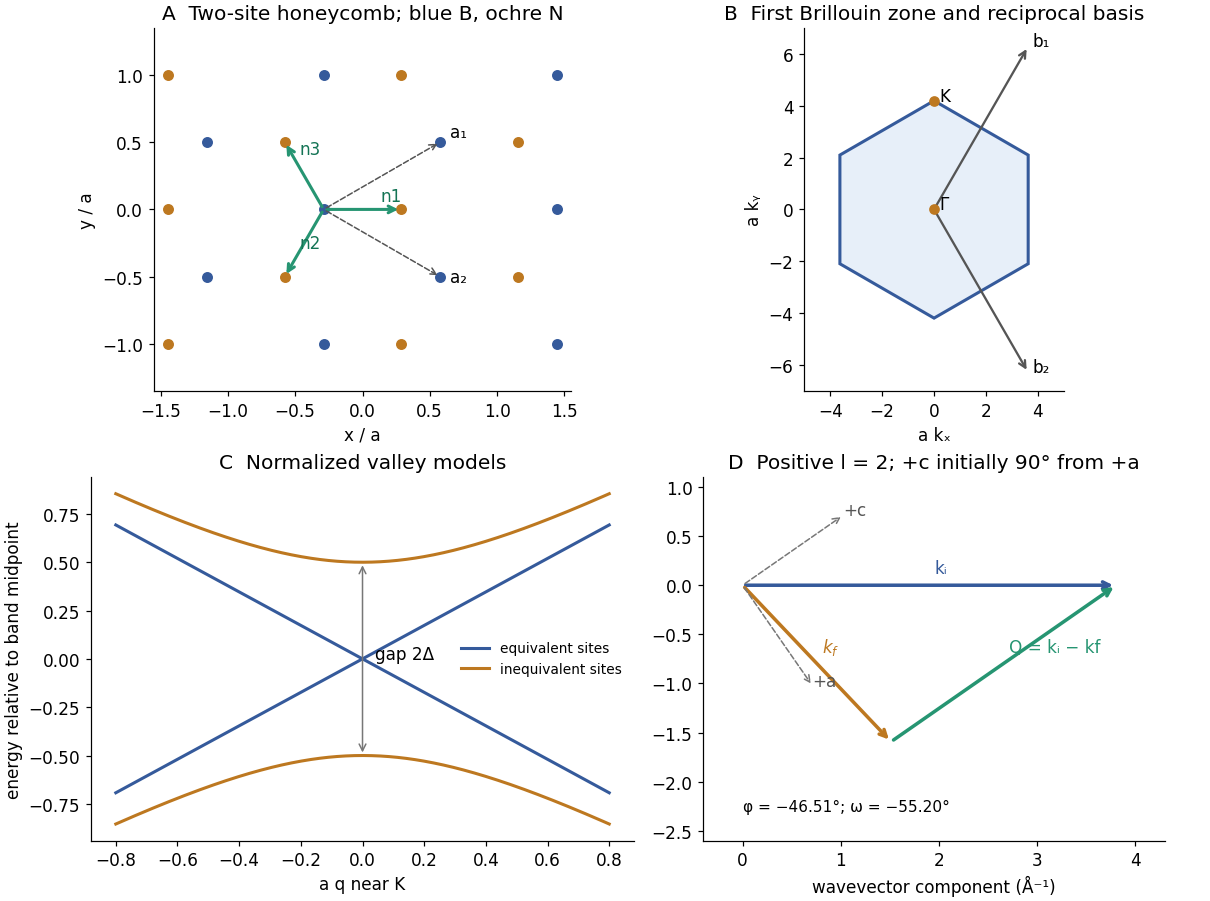
Honeycomb geometry, reciprocal-space hexagon, sublattice band gap and a signed neutron-scattering triangle
. Original calculations and schematic geometry. Lattice panels use ; the band panel compares normalized two-sublattice models. The neutron panel uses the explicit signed-axis convention of Question 1(c)(ii). Details.
The vectors from the B atom to its three nearest N neighbours can be chosen asIndeed , and . All three have length . Repeating the two-site basis over produces the honeycomb pattern in the first panel of the original figure in solution.
Solving givesThe first Brillouin zone is the Wigner–Seitz hexagon of this reciprocal lattice. Its vertices are and , with independent signs in the latter set. The centre is ; one inequivalent corner is , with . Corners related by a reciprocal lattice translation are equivalent, leaving two inequivalent valleys.
A linear combination of atomic orbitals expands a crystal wavefunction in localized orbitals on all sites,Here labels the basis site, the retained atomic orbitals and . For the two-band model retain one relevant orbital on each B or N atom, usually the out-of-plane orbital, and neglect other orbital manifolds. Define normalized Bloch sums for cells,Then . Bloch periodicity puts the same two coefficients in every cell. We adopt the stated orthonormality, neglect longer-range hopping, and approximate the diagonal matrix elements by the supplied atomic energies . More generally the crystal environment shifts these on-site energies, so equality with isolated-atom expectation values is an additional tight-binding approximation.
For equal real nearest-neighbour transfer integral , this phase convention givesThe secular determinant is . ThusSince , this is the requested algebraic form. A hopping-sign convention or rephasing of the Bloch sums changes off-diagonal phases but not these eigenvalues. Explicitly,
At a valley , . For h-BN the inequivalent sublattice energies therefore leave the direct two-band gapGraphene's equivalent carbon sites instead have in this model, so the two bands touch at the valleys. Near a valley, : graphene has approximately linear, gapless Dirac cones while h-BN has gapped band edges. The model panel in the original figure in solution displays this distinction.
First, undoped h-BN is an electrical insulator with thermally suppressed carriers, whereas neutral graphene is a zero-gap semimetal whose transport is readily changed by gating. Disorder, temperature and contacts still affect its measured conductivity. Second, h-BN suppresses interband absorption below its large gap and is transparent over much of the visible range, whereas graphene permits low-energy interband absorption unless occupations block it. A quantitative optical threshold in real h-BN also involves additional bands and strong excitonic effects; a two-orbital model should not be presented as a numerical prediction of its complete optical spectrum.
Angle-resolved photoemission spectroscopy illuminates a surface with photons of known energy and measures the kinetic energy and emission direction of the escaping electrons. Referencing the initial binding energy to the Fermi level givesHere is the sample/analyser work-function reference appropriate to the calibrated energy scale, and is the emission angle from the surface normal. Parallel crystal momentum is conserved modulo a surface reciprocal lattice vector; measuring two angular coordinates maps the two in-plane momentum components.
Sweeping angle and energy traces the occupied spectral weight and its dispersion. In a quasi-two-dimensional sheet, no detailed free-electron model of the perpendicular final-state momentum is required to map the in-plane bands. Peaks reflect the occupied single-particle spectral function, multiplied by Fermi occupation and photoemission matrix elements and broadened by finite lifetimes and resolution. Ordinary photoemission does not directly measure empty conduction bands; a gap may need complementary information. A clean surface, vacuum and charge control are especially important for an insulating specimen.
Use the explicit convention , counting every bond once and taking dimensionless spins of length . On the simple cubic lattice there are six nearest and twelve face-diagonal next-nearest neighbours.
For type I all six nearest bonds are antiparallel and all twelve next-nearest bonds parallel, so . Choose the parallel direction of type II as . It has two parallel and four antiparallel nearest bonds, and four parallel face diagonals but eight antiparallel diagonals. Thus andConsequently, for the stated antiferromagnetic exchanges,This comparison is also consistent with the full classical spiral energy. With ,It is affine in each , so some minimum occurs at a cube vertex, giving the competing collinear states above. At the boundary, the coefficient of vanishes for , producing the larger degeneracy and permutations. It is not an isolated two-state crossing. The first panel of the model figure below shows the competing energies.
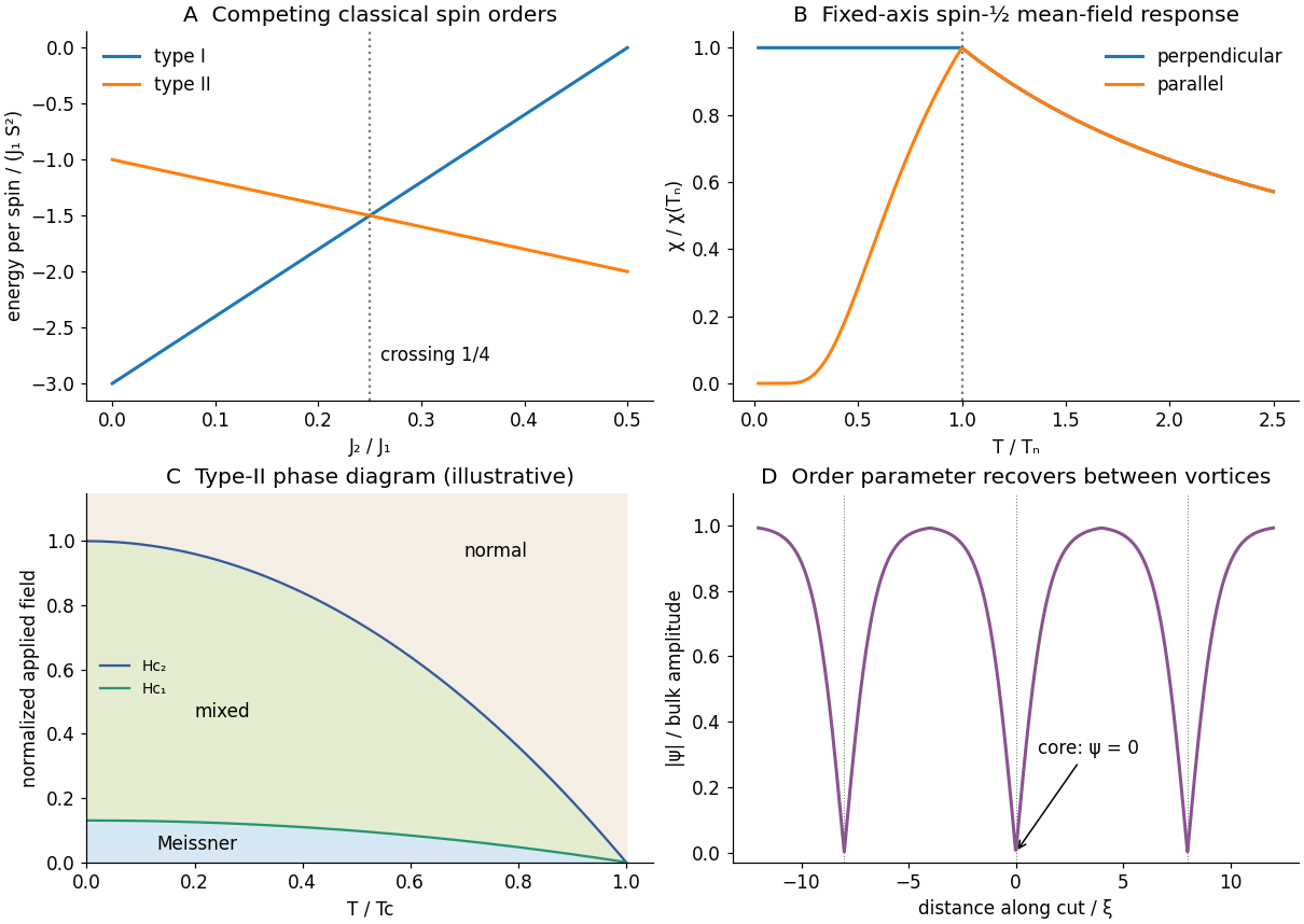
Competing antiferromagnetic energies, mean-field susceptibilities, a type-II phase diagram and vortex cores
. Original illustrative models. Susceptibilities use spin-one-half mean-field theory, fields in the phase diagram are normalized, and the order-parameter profile is a schematic cut through separated vortex cores. Details.
For type I, a magnetic unit cell uses the magnetic Bravais translations , and . They form an FCC lattice with conventional cubic parameter . A two-spin basis is an up spin at and a down spin at , or fractional conventional coordinates and . Every translation preserves the parity of .
At , the FCC translation sum allows all integers or all half-odd-integers. The spin basis contributes , which removes the integer set and leavesEquivalently the spin field is , so magnetic Bragg peaks are nuclear reciprocal vectors shifted by .
For type II with parallel spins along , use , and as magnetic translations: a primitive tetragonal cell with side lengths , containing an up spin at zero and a down spin at . The reciprocal translations have both integers or both half-odd-integers, with integer. The same basis factor removes the integer- set:This also follows from . Other domains permute the three coordinate directions. A magnetic neutron cross section further multiplies these lattice conditions by the magnetic form factor and by the component of ordered moment perpendicular to ; that polarization factor can suppress an otherwise allowed peak.
Keep the once-per-bond Hamiltonian convention of part (a). Let each sublattice magnetization be its magnetic moment per total physical volume, so the density of B-sublattice spins is . Writing their moments as fixesThe exchange energy of one A spin is , givingA convention using per bond would double this coefficient; defining magnetization per sublattice volume instead changes its normalization. The definitions above make the total magnetization .
For equal fixed sublattice magnitudes , put and , with the external field along . The effective A-site field is . Its alignment with requires , soThe last equality uses the externally imposed vacuum field and neglects demagnetizing corrections. Canting costs exchange energy but need not change the magnitude of either sublattice moment. The result holds before saturation and assumes the ordered axis is maintained when defining a transverse response.
Below , a small perpendicular field produces canting of the two ordered sublattices. In the isotropic two-sublattice mean-field model, the induced component is : the reduced ordered moment at higher temperature tilts more easily and the two effects cancel. Thus remains constant until the transition.
A field parallel to the maintained ordering axis instead increases the magnitude of one sublattice magnetization and decreases the other. At zero temperature saturated localized spins have essentially no such amplitude response in this model, so . Thermal population changes make it easier to redistribute the longitudinal moments as temperature rises, giving the growing longitudinal susceptibility that meets at . These directions presume the domain or a weak anisotropy fixes the ordered axis; in a perfectly isotropic freely rotating sample the Néel vector can reorient.
Above there is no chosen magnetic axis, so the response is isotropic. Antiferromagnetic correlations oppose uniform magnetization, giving the mean-field Curie–Weiss formAt it equals , consistent with the transverse branch; at large temperature it decreases as . A negative Weiss temperature characterizes this uniform antiferromagnetic response, rather than a ferromagnetic divergence at positive . The illustrative mean-field curves in solution make these limits visible.
Seek the steady forced displacement as . The oscillator equation givesFor ion pairs per volume, the ionic polarization is . Add the electronic polarization , assumed frequency-independent over this infrared range. The complex relative permittivity is thereforeFor a longitudinal free oscillation without external free charge, and the longitudinal electric field requires in the lossless limit. HenceEliminating the microscopic oscillator strength givesHere denotes the undamped longitudinal frequency; with finite damping the zero is at a complex frequency. The sign of the imaginary term follows the stated convention and gives positive absorptive for , . At zero frequency the same model yields the Lyddane-Sachs-Teller relation . The high-frequency limit here is above the phonon resonance but below electronic resonances, not arbitrarily high photon energy.
At normal incidence from vacuum the reflectivity iswith the passive branch of the complex refractive index. Below the optical resonance the real permittivity rises towards its pole and reflectance increases. Between the TO and LO frequencies, the lossless permittivity is negative; the wave is evanescent and the reflectivity is unity in that idealization. Finite damping rounds and reduces this reststrahlen band. Above the LO edge, positive permittivity returns and reflectivity can become very small when the refractive index is near one, before rising towards its electronic-background value.
Reading the surviving source graph to its available precision givesThese are band-edge estimates, not a high-precision damping fit. The minimum immediately above the band is not exactly the LO zero: for zero damping occurs at .
The high-energy plotted tail near has . Ignoring residual phonon dispersion gives and . Correcting with the finite-energy oscillator ratio givesThus a background of order – is supported; equating the still-dispersive tail exactly to the asymptotic background would slightly underestimate it. The original model curves below use these approximate energies, without copying or fitting individual source data points.
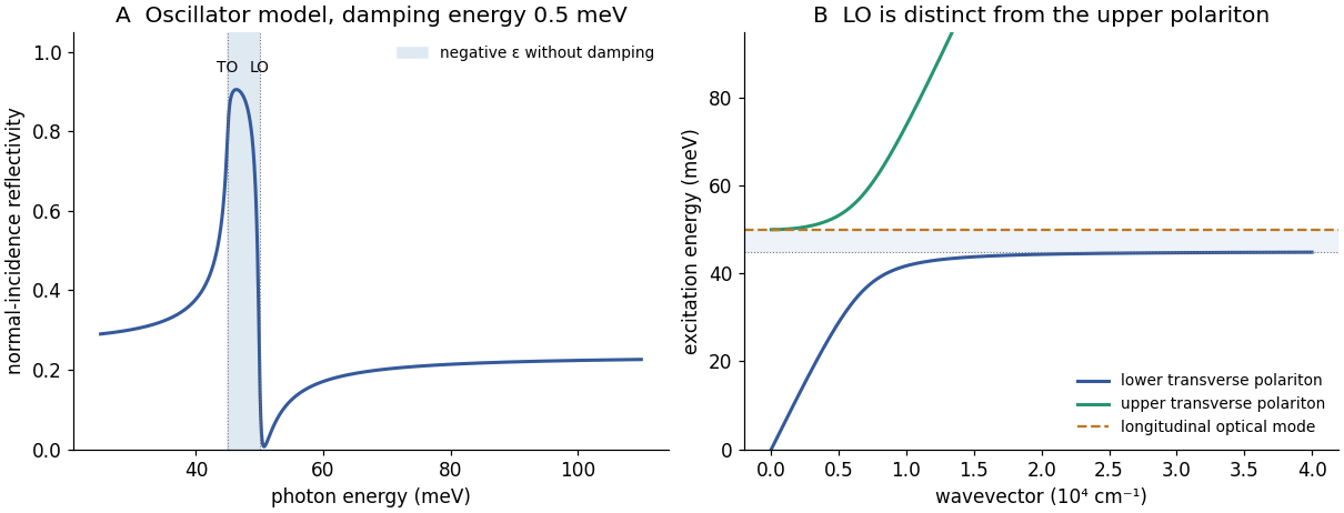

For a transverse electromagnetic plane wave in a nonmagnetic medium, Maxwell's equations give . Set damping to zero and define . Substitution yieldsso . Therefore the two phonon polariton branches areTake the nonnegative square root for the positive physical frequencies. At , and . At small wavevector the lower branch is photon-like with velocity ; at large wavevector it approaches from below. The upper branch ultimately becomes photon-like with velocity . There is no real propagating transverse branch with frequency strictly between and in this lossless bulk model. Coupling changes the eigenmodes from a bare photon crossing a flat oscillator into mixed normal modes.
In Raman scattering, the photon transfers and to a collective excitation. Changing scattering geometry selects different and probes its dispersion.
The open circles rise and then flatten near : they trace the lower transverse phonon polariton branch. It is strongly dispersive on its photon-like side, then becomes predominantly TO-phonon-like and approaches the TO energy at larger wavevector. The open triangles stay near and are the nearly nondispersive longitudinal optical phonon. Longitudinal motion creates its own polarization field and is shifted above the transverse resonance. It does not hybridize with a propagating transverse photon in the same way, and it should not be misidentified as the upper transverse polariton branch, which rises with wavevector. Raman tensor and polarization selection rules determine which excitation is visible.
Scale qualification: the source horizontal label appears to print . Taken literally, one plotted unit would have vacuum photon energy only , inconsistent with the observed tens of meV and the dispersive polariton. The physically compatible scale is of order ; the qualitative branch identification does not require silently treating the printed negative exponent as correct. The original model figure in solution explicitly labels its calculated wavevector scale.
In weak-coupling BCS theory, a useful scale isHere the phonon spectrum sets the attractive-interaction cutoff, is the consistently defined Fermi-level density of states and the effective pairing attraction after repulsion is accounted for. Light hydrogen supports high vibrational frequencies; strong electron–phonon coupling and favourable metallic density of states can raise . Pressure changes bonding, phase stability, electronic structure and phonon frequencies. It is not simply an independent multiplier in this expression. In a real strongly coupled hydride, Eliashberg theory uses the full spectral function and a screened Coulomb pseudopotential; the elementary exponential is a mechanism guide rather than a controlled quantitative fit to .
Measure a four-terminal resistance that falls below the instrumental bound, and test that a magnetic field suppresses the transition. Independently detect diamagnetic screening and, where feasible, field-cooled flux expulsion or an AC susceptibility signal with controlled cell background. A resistance drop alone can reflect contact changes or a filamentary path; a consistent magnetic response is important evidence for superconductivity. A reproducible isotope shift upon replacing hydrogen by deuterium tests the involvement of lattice motion, although it is not by itself proof of superconductivity.
Extreme-pressure samples are microscopic and enclosed in a diamond-anvil cell. Reliable separate electrical contacts, homogeneous pressure, pressure calibration during cooling, chemical stability and the tiny magnetic signal relative to the anvils and gasket are practical difficulties. Structural identification matters because a sulfur-rich hydrogen compound formed under pressure need not retain the starting stoichiometry.
Historical correction: the original primary report associates the transition with pressures near , while roughly is the metallization scale, not that same transition point. The printed pairing of with should not be treated as an established measured pair. The statement about the highest conventional transition temperature is also a historical statement in this 2018 examination.[ref]
Conventional superconductivity at 203 kelvin at high pressures in the sulfur hydride system by A. P. Drozdov and others. Primary 2015 report: metallization near 90 GPa, high-temperature transition near 155 GPa, transport, magnetic and isotope evidence
For an ideal long specimen with negligible demagnetizing field, the Meissner state has , so . A type-I superconductor retains this response up to its thermodynamic critical field and then enters the normal state, where the small normal magnetic response can be neglected. Nonzero demagnetizing fields can create an intermediate state and broaden the measured transition.
A type-II superconductor is fully screening only below . Between and , magnetic flux enters as quantized vortices and the reversible magnetization remains diamagnetic but decreases in magnitude towards zero at . Above the bulk is normal. Ginzburg–Landau theory distinguishes the types at , not at ; the later condition in the source merely restricts its estimate.
The – sketch has two increasing-width regions below : Meissner below the lower boundary, mixed vortex state between the two boundaries, and normal state above the upper boundary. Both critical fields vanish at . The phase-diagram panel of the original figure in solution shows this topology; its normalized field curves are illustrative, not a fit to the source magnetization loop.
The displayed horizontal variable is in tesla. The source formulas written with a flux quantum actually have the dimensions of magnetic flux density, so define and when applying them:From the onset of curvature away from the low-field line in panel A, is roughly with uncertainty of order . Panel B's branches approach the normal background over approximately –; use as a coarse central estimate. Resolving irreversible loop closure from the true thermodynamic upper field, and correcting demagnetization, would require better data and geometry. These readings support scales, not precise material constants.
The upper field givesThe leading-log critical-field inversion starts by dividing the two field formulas to eliminate :The large- solution is , henceThe penetration-depth range is an indicative graph/model scale, not a propagated confidence interval. There is a mathematical ambiguity worth making explicit: rises from zero at one, peaks at , then falls. The same central ratio also gives and , so the printed restriction alone does not select a unique solution. The leading-log lower-field formula is intended for appreciably large , which motivates the branch; near one it needs the omitted core-energy correction. Even the larger-branch estimate has systematic uncertainty from that approximation.
is the London penetration depth, the magnetic screening scale, while is the superconducting coherence length, the recovery scale of the superconducting order parameter after spatial suppression. In the mixed state the complex order parameter vanishes in vortex cores of radius of order , recovers between separated cores and winds in phase by around each singly quantized vortex. Currents and magnetic field spread over scale ; vortex density grows with the mean internal field according to . Near cores overlap and the order-parameter amplitude becomes small throughout the sample. A schematic core profile appears in solution.
The hysteresis is not the reversible equilibrium magnetization: defects pin vortices, so entry and exit leave different spatial flux distributions. Macroscopic currents oppose changes in flux, trapped vortices give remanence, and depinning and creep depend on history and temperature. Surface barriers can also contribute. The loop width probes an irreversible current scale, but its conversion to current density additionally needs sample geometry and an appropriate critical-state model.
For a long cylindrical wire carrying axial current , Ampère's law gives at its surface. With , the current resides mainly in a shell of thickness . If “critical” denotes the first equilibrium entry of vortices in an otherwise Meissner wire, set :The dependence on is necessary because no numerical radius is supplied. The local surface current density at this entry scale is different:Its conversion to the cross-section average is . Treating the shell current density as uniform over the entire thick wire would overestimate its total current by .
Meaning of a maximum: in a type-II material, first vortex entry need not be the measured dissipative transport limit. Pinned vortices can sustain greater current, whereas freely moving vortices generate voltage. The hysteresis loop indicates pinning, but no geometry-dependent pinning force or transport criterion is given, so a unique practical maximum cannot be deduced solely from and .
For comparison, the intrinsic homogeneous Ginzburg–Landau depairing scale follows from . Maximizing at givesThis is a local, approximately uniform-flow theoretical scale, not the average current density throughout a thick self-field wire. Surface barriers, nonlinear screening, vortex motion and temperature determine how that scale relates to its actual critical current. Thus the entry estimate, local shell density and intrinsic depairing limit answer distinct physical criteria; the source's word “maximum” does not supply the missing pinning information.
A sufficiently clean two-dimensional electron gas at low temperature in a perpendicular magnetic field has quantized orbital Landau levels. In the integer quantum Hall regime, the longitudinal resistivity is nearly zero while the Hall resistance has plateauxThe Hall sign depends on carrier charge and lead convention. Fractional plateaux can occur in strongly interacting states, but the following single-particle counting and calibration use the integer effect.
One resolved spin branch of a Landau level has one state per flux quantum : in area , its guiding-centre degeneracy is for positive . Defining the nominal filling factor as the number of electrons per available orbital state givesThe same count follows in Landau gauge: a increment in moves the orbit centre by , giving states. Include each spin branch separately; an unresolved spin-degenerate orbital level contains twice this count, and common plateau indices are then even.
Plateau qualification: as defined by density is continuous when changes at fixed . The integer plateau index can remain unchanged over a field interval because localized states accommodate the changing occupation. Therefore is not an exact identity across an entire plateau. It is the ideal filled-level relation, often used approximately at a suitable plateau centre; confusing the nominal filling with the plateau index would contradict fixed density.
The plateau resistance realizes the von Klitzing constant , divided by a known integer. A four-terminal Hall measurement with negligible longitudinal voltage and contacts in the quantized regime supplies a reproducible resistance reference, which can be compared to other resistors using precision bridges. Its robustness comes from the quantized transport state, not from measuring the Hall bar's width accurately.
The Hall-plateau voltmeter calibration is obtained as follows. Let be a plateau height in displayed units after any voltage offset is removed, with identified integer plateau index . The true Hall voltage is , so the calibration factor would beThe nominal current is . If several plateau heights are available, their inverse-integer ratios help identify indices and a fit of against can separate a constant offset from the gain. Reversing magnetic field and antisymmetrizing the voltage also removes an even offset. A unique absolute index should not be asserted solely from an unspecified sequence of steps.
For an established exact integer and independent current and height errors,The current alone contributes relative uncertainty; it is a common calibration uncertainty and does not average away by fitting more plateaux. Voltage-offset uncertainty and deviations from quantization must also be included where relevant. The width cancels because the Hall voltage divided by current is a sheet Hall resistance; it would enter the transverse electric field, not this calibration.
TODO — missing source data: the held PDF's last-page stream refers to an absent
/Im6 graphic, and its recovery log reports an unknown XObject. The supplied TeX records the same source gap. No plateau heights, labels or axis values survive, so neither a numerical nor a unique can be read. The numerical voltmeter calibration and its complete graph-reading error cannot be supplied without that graph; the formula and known current contribution above are determined.As magnetic field grows from zero, a clean two-dimensional electron gas first has an ordinary finite longitudinal resistivity, then develops Shubnikov–de Haas oscillations as broadened Landau levels pass the chemical potential. Thermal and disorder broadening obscure the low-field oscillations; their visibility grows when the level spacing exceeds those broadening scales. In a well-developed integer quantum Hall regime, has minima close to zero on Hall plateaux and maxima during transitions between them, when extended states cross the chemical potential. Detailed peak heights and envelopes depend on disorder and scattering and are not fixed by quantization alone.
At fixed density the nominal filling is , so level-filling features are approximately periodic in , with period for resolved spin levels or for an unresolved spin pair. Increasing lowers the filling; spin splitting can create additional odd-index features. The original schematic below shows these relations without pretending to reconstruct the missing data.
TODO — missing source graph: the actual – positions and integer plateau labels require or surviving plateau fields from part (b). Neither is provided independently. Thus a uniquely labelled field-axis sketch for this sample cannot be completed. The following DOS diagram distinguishes extended centres and localized tails generically; its chemical-potential markers are illustrative and do not stand for the requested 8 T or 10 T assignments.
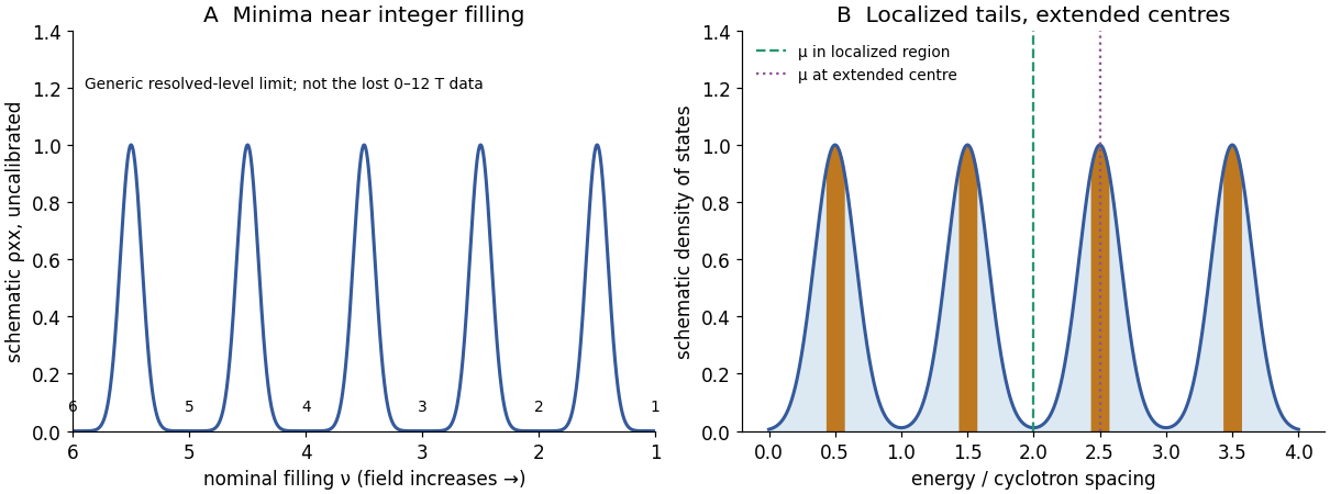
Generic longitudinal oscillations and broadened Landau levels without inventing the missing Hall data
. Original qualitative illustration. The horizontal filling scale is dimensionless and is not a reconstruction of the missing 0–12 T graph. Chemical-potential positions in the DOS panel illustrate two regimes, with no assignment to 8 T or 10 T. Details.
At , the nominal filling isA labelled density-of-states picture has disorder-broadened peaks at these orbital and spin energies, localized tails and extended states near their centres. A chemical potential in the localized region corresponds to a Hall plateau and small longitudinal resistivity; passing through an extended-state centre corresponds to a transition.
TODO — missing density/plateau assignment: there is no basis for choosing one of those positions at 10 T without the missing Hall graph. For example gives nominal , whereas gives . In an ideal resolved-level picture the first can put the chemical potential between filled levels, while the second leaves a level partly filled. Both are compatible with the surviving current and width, demonstrating why the requested placement is undetermined.
At ,The cyclotron spacing is , smaller than at 10 T, and each resolved level's degeneracy per area is also reduced by . Thus the same carrier density occupies more levels. This ratio is determined without the missing graph, but it does not specify whether the chemical potential lies in a localized tail or an extended-state centre.
TODO — missing density/plateau assignment: a numerical index and chemical-potential marker at 8 T require the unavailable density information. For example the first illustrative density in part (i) gives , while instead gives . These produce different schematic placements even though both satisfy every surviving sample parameter. Unresolved spin degeneracy and disorder add further qualifications; no unique 8 T label should be invented.
A perfectly clean two-dimensional system has sharply degenerate Landau levels and integer filling only at isolated fields for fixed density. Real disorder broadens each level into a band, with states localized in the tails and extended states near its centre. When the chemical potential moves through a localized region, changing field can change the occupation of those localized states without changing the number of conducting extended channels. The Hall conductance then remains and the Hall voltage at fixed current remains over a finite field interval.
In the same regime, separated edge channels and localized bulk states suppress dissipative backscattering, so is very small. At a transition the chemical potential reaches the next band of extended states; longitudinal conduction rises and the Hall conductance changes to another integer. This is a mobility-gap explanation: a plateau does not require the density of states itself to vanish, nor does it require the carrier density to grow linearly with field. Low temperature, sufficient mobility and suitable contacts are needed to resolve it.
This physical explanation is determined by the surviving question text. Particular measured plateau heights and widths cannot be quoted because the source graph is absent, as recorded in part (b).
Articles by others on the same topic
There are currently no matching articles.