Sylvester's law of inertia says that any real quadratic form has coordinates in which it is a sum of positive squares minus negative squares, with unused coordinates, and that the numbers are invariant under every invertible linear change of coordinates. Its rank is ; its signature of a quadratic form is commonly , with also called its signature pair.
The symmetric matrix here is , where and . On the line spanned by , has eigenvalue . If , then , so that the orthogonal complement has eigenvalue with multiplicity . Thus the off-diagonal all-ones quadratic form hasFor the form vanishes, so rank and scalar signature are both zero, with inertia . Including this case is necessary because the distinguished eigenvalue then becomes zero.
A Euclidean domain is a commutative integral domain with a function such that, for with , there are satisfying , where either or . One may also impose the usual monotonicity for nonzero ; the example below has it.
The integers form a Euclidean domain that is not a field. Use . Integer division by supplies a remainder with , and changing the sign of the quotient handles negative . The integers are an integral domain, while has no multiplicative inverse in them. This verifies both the Euclidean property and the failure to be a field.
The structure theorem for finitely generated modules over a principal ideal domain applies because every Euclidean domain is a principal ideal domain. In invariant-factor form, every finitely generated module over such a domain has a decompositionwhere the are nonzero nonunits, , and either list of summands may be empty. The free rank and the invariant factors are unique up to multiplication of each by a unit. Equivalently the torsion part is a direct sum of cyclic modules with prime-power annihilators. The nonunit convention omits zero summands .
Change the generators to , and . This is an invertible integer change of generators, since , , . The relations become and , with no relation involving . ConsequentlyThis is already the invariant-factor order required by the structure theorem for finitely generated modules over a principal ideal domain, because . The inverse change of generators shows that there are no hidden extra relations.
Uniform convergence of to on an interval means that for every there is such that for all and every . Equivalently . The same must work throughout the interval, unlike pointwise convergence.
For completeness, continuity is preserved: choose with uniform error below , and use continuity of at a given to make . The triangle inequality then gives . Thus each function involved in the integral is continuous on the closed interval and Riemann integrable. The estimateproves convergence of the integrals by uniform convergence. When both integrals are zero.
For each fixed , , so the only possible limit is zero. But taking gives for every . In fact the supremum of over the interval is infinite for each . Thus the convergence is pointwise but not uniform; uniform convergence cannot be inferred from convergence at each fixed point.
The pointwise limit is the constant function . For , the inequality for givesHence the sequence converges uniformly to one on . Its exact supremum error is , although the supremum is not attained on the open interval. Compactness of the interval is not needed for this uniform convergence bound.
The equation implies . Its intersections with and are disjoint, nonempty subsets open in the subspace topology, and together cover the entire surface. They therefore form a separation, proving the surface is disconnected. More precisely its two sheets are ; each is homeomorphic to the connected plane by projection, so these are exactly its two connected components.
Factorization gives or . Each point can be joined to the origin by a straight segment lying on its own line. Two such segments join any pair of points, so the union is path-connected and hence connected. Alternatively it is the union of two connected lines with a common point.
The map is a continuous surjection from the path-connected plane onto this surface. It is a homeomorphism because coordinate projection is its continuous inverse. Thus the paraboloid is path-connected and connected. Explicitly, lifting any straight planar segment by this map produces a path on the surface.
At a constrained stationary point where , every tangent direction to is orthogonal to . Vanishing of the directional derivative of in all such directions forces for a Lagrange multiplier . Solve these equations together with the constraint, then check the candidates and any singular or limiting cases for minima or maxima.
Let a closed cylinder have radius and height , with fixed . Its area is and the constraint is . The Lagrange multiplier equations giveThe second yields ; substituting into the first gives . Thus the minimum-area closed cylinder at fixed volume hasTo prove it is the global minimum, eliminate to obtain . Its derivative is , negative before the displayed radius and positive afterwards; the area tends to infinity both as and as . This establishes uniqueness and rules out limiting smaller areas.
Take the divergence of the Ampere-Maxwell law and use Gauss's law . Since the divergence of a curl is zero, this gives the charge continuity equation . Uniform conductivity and Ohm's law imply . ThereforeThe spatially uniform initial density stays uniform in the interior; is the charge relaxation time.
Denote the cylinder radius by . Cylindrical symmetry makes the interior electric field radial. Gauss's law on a coaxial cylinder of radius and length gives . ThusThe current does not disappear at the interface: the vacuum conducts no current, so charge accumulates on the cylindrical surface. Initially taking the charge to be the stated volume charge alone, its surface charge density satisfies , giving the charge relaxation in an isolated conducting cylinder lawThe total enclosed charge per unit length is . Consequently the exterior electric field isindependent of time. The boundary jump obeys , as it must. Applying Gauss's law to the decaying volume charge alone would incorrectly predict a decaying exterior electric field and violate electric charge conservation. The vector formulas also specify the inward direction if .
Write for coordinates in the rest frame of and for those in the rest frame of . The Lorentz transformation is and . Along the worldline of , . Cancelling gives , so the relativistic velocity-addition formula yieldsApply the same Lorentz transformation between the rest frames of and to . Its velocity in the former is . Substitution simplifies toHere and the formulas use signed collinear velocities. In the given positive-direction setting they are positive speeds. The limit recovers ordinary addition, providing a check on both expressions.
A material derivative measures the rate experienced by a moving fluid particle. If its position is with , the chain rule for any scalar field givesHence the operator is , and the material derivative differs from the time derivative at a fixed spatial point.
In the steady temperature problem and the transverse velocity vanishes. Thus at each fixed ,Integrating in and applying the inlet value givesA particle's travel time from the inlet is , so the formula is also the exponential decay along its characteristic curve. For fixed the temperature tends to zero near either wall, because the travel time becomes large. No value at is imposed by an inlet condition there, since the wall velocity is zero and the stated channel is open in .
A cut of a flow network of a directed flow network is a partition with the source in and the sink outside it. Its cut capacity is . Summing flow conservation over all vertices of cancels every internal edge and gives the flow value as outgoing flow minus incoming flow across the cut. Incoming flow is nonnegative and outgoing flow is bounded by capacity, soThis is weak duality for the maximum-flow problem; no converse theorem is needed for the upper bound.
For this grid, use . It contains but not . An adjacent edge can leave only by reaching the diagonal. Each of the three interior diagonal vertices has two incoming crossing edges and each endpoint has one, making eight edges. Every crossing edge has capacity one. Thus the diagonal cut in a nearest-neighbour lattice flow has capacity eight.
Here is a feasible flow of value eight. Send one unit on each of the following directed paths, and zero on every edge not used. In this list abbreviates the vertex :Every path conserves flow at its intermediate vertices. To check the capacities without hiding a feasibility assumption, group used edges by capacity: the capacity-one edges are traversed at most once; the capacity-two edges at most twice; the capacity-three edges at most three times; the capacity-four edges at most twice. Shared source edges , , carry units, and the corresponding three sink edges carry . The diagram displays every positive edge flow beside its capacity. Thus all constraints hold and the matching cut proves
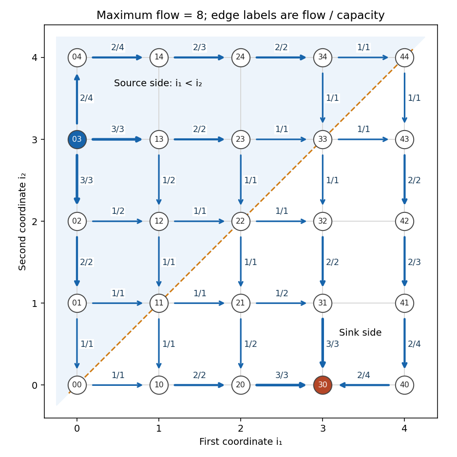
Feasible eight-unit grid flow with edge labels showing flow over capacity and the diagonal cut of capacity eight
. Details. 
The monomials are linearly independent and span, so . Use the factorial monomial basis for polynomial differentiation , . Direct differentiation gives . HenceIndeed every has the Taylor expansion ; evaluation on the proves independence of the functionals. Derivative orders include zero. If one uses a convention excluding zero from , must explicitly be included, since all positive-order derivatives annihilate constants and cannot span the dual space.
Differentiation satisfies and for . With column vectors of coefficients, its matrix has entries if and zero otherwise, for indices :The dual map is , not a conjugate-linear adjoint. Thus for and . Therefore in the corresponding dual basis. For both matrices are the one-by-one zero matrix.
Let be the set of all subsets of with elements. First show that is not divisible by . In the polynomial ring over the field of elements, , since the intermediate binomial coefficients are divisible by . Iterating givesComparison of coefficients of yields .
Let act on by left translation. Because its orbit sizes sum to a number not divisible by , some orbit has size prime to . Choose a subset in that orbit, with stabilizer . The orbit-stabilizer theorem gives the orbit size , so . On the other hand acts freely on the elements of : if , cancellation in the group gives . Every -orbit in therefore has elements, and divides . Sinceand the second factor has no factor of , the first must contain all . Hence , proving the first of the Sylow theorems. This is Sylow existence by subset action and includes the trivial case .
The remaining Sylow theorems state that every -subgroup of a finite group is contained in a Sylow subgroup, and that all Sylow -subgroups are conjugate. If with and is the number of Sylow -subgroups, thenIn particular if and only if that Sylow subgroup is a normal subgroup.
Relabel the two primes so that . By the Sylow theorems, the number of Sylow -subgroups divides , so it is either or . But and , ruling out . Thus there is a unique Sylow subgroup of order , which is a normal subgroup. It is nontrivial and proper because . Consequently no group of order is simple. No additional assumption on divisibility of by is required.
The second fundamental form records the normal component of second-order bending of the surface. For a surface curve , the terms containing and are tangent and thereforeThus on a unit tangent direction it gives the normal curvature; for a general coordinate direction the normal curvature is the ratio of the second to the first fundamental form. Equivalently the quadratic part of displacement out of the tangent plane is one half of this form. Reversing the chosen unit normal changes its sign.
Now suppose . Differentiate . This givesAlso differentiation of gives . The parametrization is regular, so form a basis of three-dimensional space. Both normal derivatives are orthogonal to this basis and hence vanish:The parameter ball is connected; integrating these derivatives along a straight segment between parameter points shows that is constant. Finally both derivatives of vanish, because are tangent. Thus the zero second fundamental form implies planar image statement isThe PDF has in the second derivative equality; the apparent in the TeX is not a distinct coordinate.
If with and , the chain rule gives , the product of a two-by-one and a one-by-two matrix. Its rank is at most one, so its Jacobian determinant is identically zero.
Conversely, continuity and give a neighborhood on which stays nonzero. The identity then implies . Therefore the smooth function satisfiesFor a graph curve with constant, the first component must have derivative zero. Thus the necessary equation isIt is also sufficient: it makes , and then .
To justify the existence through every nearby point, choose a closed rectangle about the origin inside . The right-hand side is smooth there, hence bounded and locally Lipschitz in . The Picard-Lindelöf theorem supplies a unique local solution through every initial point in a smaller open rectangle . The boundedness of and a positive distance from the smaller rectangle to the outer boundary permit a common sufficiently short time interval about each on which the solution stays in . Each point of therefore lies on one of these graph curves, and the preceding chain-rule calculation proves that is constant along it. This proves rank-one level curves from a characteristic differential equation using local ODE existence. The curves are local in their time parameter; no unjustified global existence for all real is required.
The intended open region lies inside the larger circle and outside the smaller one. The two circles are tangent at zero, a boundary point, so is holomorphic throughout the region. For a circle , its equation is , which becomes . The side inside that circle becomes . Hence the tangent-circle crescent conformal map begins withThe affine coordinate sends this strip bijectively to . Exponentiation is then a conformal bijection to the upper half-plane: its argument ranges strictly from zero to , and the inverse logarithm has that unique argument. Finally is a Cayley transform between the half-plane and disk onto the unit disc, since for its modulus is less than one and the inverse is . As , a complete answer isEvery stage has nonzero derivative and is one-to-one onto its indicated range. The denominator cannot vanish in the upper half-plane. Unlike a region between disjoint nested circles, this tangent crescent has no enclosed hole, so there is no annulus obstruction to mapping it onto a disc.
For , substitution in the unnormalized equation gives . For , the remaining expression is . Thus an independent second solution is . Their Wronskian is , nonzero on .
The left boundary solution is , since ; the decaying right solution is . A Robin half-line Green function from left and right solutions must be continuous at , while its derivative jumps by one because the leading coefficient of is one. These conditions giveThereforeThe two values agree at , and . Each branch solves the homogeneous equation and its relevant boundary condition, so these checks prove the distributional identity rather than merely postulate the kernel.
Integrate this Green function against the forcing . Splitting at givesIt has and decays at infinity. Direct substitution gives . Uniqueness follows because a decaying homogeneous solution must be a multiple of , and its left boundary condition would require , forcing .
For a bound state take and set . Substitution into the radial equation and cancellation of the common exponential giveSeek a power series with . Equating coefficients of yields the polynomial construction of hydrogen S states recurrenceFor any integer , choose . The numerator vanishes at , while it is nonzero for , so is a nonzero polynomial of degree . Therefore is continuous at and decays exponentially as . The three-dimensional normalization integral isIt is finite near zero because is bounded, and finite at infinity because an exponential dominates every polynomial. Multiplying by its positive reciprocal square root gives a normalizable, nonzero wavefunction. The recurrence ensures the differential equation for ; at the singular endpoint the regular continuous extension has , so the potentially singular coefficient cancels. No nonexistent value of at zero is substituted.
Since , the choice of givesFor , the normalized example is . For , is proportional to . These illustrate the polynomial-times-exponential Coulomb bound states produced for every required energy. The radial derivative at the origin is generally nonzero, a Coulomb cusp consistent with the requested continuity.
For steady electromagnetic fields, Maxwell's equations give and . Introduce a magnetic vector potential with and the permitted Coulomb gauge . The vector identity for the double curl then gives . For localized currents and the decaying solution,Here follows from harmonicity away from zero and the inward flux of the radial derivative through a small sphere, whose magnitude is one. It verifies the vector Poisson solution componentwise. Moreover steady electric charge conservation gives ; integration by parts confirms the stated potential is divergence-free. Taking its curl, using , proves the Biot-Savart law:The zero-field condition at infinity selects the magnetic field produced by these currents, excluding an externally imposed homogeneous magnetic field.
At the origin write the source point as . Its current is , so the numerator of the Biot-Savart law is . The radial term cancels after angular integration. Using givesThe inner integral is , as is verified by differentiating . HenceFor , its magnitude is ; it points along for positive azimuthal current , and along for . The limit is , agreeing with direct integration of the infinitely long cylindrical current distribution.
For node , let be the Lagrange interpolation polynomial with . It has degree , so has degree . The Gaussian quadrature with nodes is exact through degree , henceThe integrand is nonnegative. Since is a nonzero polynomial, it is nonzero on some open subinterval; the positive weight has positive integral there. Consequently for every node. This proves the positive weights of Gaussian quadrature property without assuming any coefficient sign beforehand.
Write , finite and positive. Exactness on the constant polynomial gives . Positivity therefore implies the uniform operator bound , and the integral has the same bound.
For a continuous and , the Weierstrass approximation theorem gives a fixed polynomial of degree with . For every , polynomial exactness gives . ThusSince is arbitrary, for every continuous . This is convergence of positive quadrature on continuous functions. The argument requires nodes in , implicit in a rule defined on all continuous functions there; otherwise their function values would not even be specified by the stated domain. Exactness alone would not provide the norm bound if arbitrarily signed weights were allowed.
Put , and let be the exact standard-normal 95th percentile. Under parameter , with standard normal. This distribution can be justified directly: the joint density of the centered observations is proportional to . An orthogonal change of coordinates with first row has unit absolute Jacobian and preserves the sum of squares. Its density factors into one-dimensional standard-normal densities, making the first coordinate standard normal.
Consider the test . Its rejection probability isincreasing in . Therefore its maximum rejection probability over the null is achieved at zero and equals . This proves it has the required test size.
To prove the uniformly most powerful test property, rather than quote the Neyman-Pearson lemma, fix any . The likelihood ratio of the full sample against isstrictly increasing in . Set . For any competing possibly randomized test with composite-null size at most , we have . Pointwise,because both factors are nonnegative above the threshold and both are nonpositive below it. Integrating givesThis comparison proves the likelihood-ratio optimality result needed here in full. Since the same critical region works for every , it proves the uniformly most powerful test property over the entire alternative.
For , the exact critical region and its quoted-table approximation areUsing the supplied rounded percentile gives . The exact cutoff uses and hence ; the rounded cutoff is the intended numerical approximation, not a literally exact size- threshold. The Gaussian distribution is continuous, so equality at the cutoff has probability zero and no randomization there is needed.
Until the first visit to zero, the positive-side chain is a nearest-neighbour random walk with upward probability and downward probability . For an integer , let , . The Markov property givesThe characteristic roots of this recurrence are and . Solving its two boundary equations gives the biased gambler's ruin probabilityA finite path that reaches zero has a finite maximum before doing so, and is counted by for every sufficiently large . Conversely each such event implies a visit to zero. Therefore these events increase to , and continuity of probability givesMore generally the hitting probability from is . The finite-boundary derivation avoids choosing an unjustified solution of the infinite recurrence.
On the negative branch set . Its outward step probability is and inward probability is . The same finite gambler's ruin recurrence as in part (a), with root , gives . Hence, following one departure from zero, the probability of returning isAt each return the Strong Markov property restarts the same excursion experiment. The probability of at least returns is , tending to zero. Thus almost surely there is a last visit to zero.
After that visit the walk remains strictly positive or strictly negative, because nearest-neighbour steps cannot change sign without crossing zero. On the positive branch it can be coupled, up to any return, to independent steps of mean . The strong law of large numbers gives a walk tending to almost surely. This conclusion remains true on the event that the excursion never returns: conditioning on a positive-probability event cannot make a probability-zero failure of the law occur. On the negative branch the mean step is , giving in the same way. Apply this at each possible departure time, a countable family, or use the Strong Markov property at the successive returns. ThereforeFinite visits to zero alone would not prove divergence on an arbitrary chain; the outward-drift argument is the additional step needed here.
One excursion from zero escapes forever on the positive branch with probability , and on the negative branch with probability . The remaining probability is the return probability . By the last-excursion direction law at a transient junction, the eventual positive escape probability isEquivalently, if denotes the desired probability, the Strong Markov property gives . The negative escape probability is , and their sum is one, as independently established in part (b).
Articles by others on the same topic
There are currently no matching articles.