Past exam of the mathematics course of the University of Cambridge / 2006 / ii / Paper 2

Use the usual positive-definite convention for binary quadratic forms with negative discriminant. Reduction by integral changes of variables of determinant one produces a form $a{x}^2+bxy+c{y}^2$ with $|b|\le a\le c$, and with $b\ge 0$ on the boundary. For completeness, replacing $x$ by $x+ny$ makes $|b|\le a$; if then $c<a$, interchange the variables, reversing one sign to keep determinant one. The new positive leading coefficient is smaller. Repeating terminates and gives a reduced form.

For discriminant $-7$, $4ac-b^2=7$ and the reduction inequalities give $3a^2\le 7$. Thus $a=1$, $b$ is odd and $|b|\le 1$, and $c=2$. The boundary convention chooses $b=1$. Hence there is exactly one positive-definite equivalence class, represented by $x^2+xy+2y^2$.

For an odd prime $p\ne 7$ represented by this form, the identity $4p=(2x+y{)}^2+7y^2$ shows that $-7$ is a square modulo $p$. Here $p\nmid y$, because otherwise $p\mid x$ and $p^2$ would divide the represented number. Conversely, if $-7$ is a square modulo $p$, choose odd $b$ with $b^2\equiv -7(\mathrm{mod}p)$. Then $(p,b,(b^2+7)/(4p))$ is an integral positive-definite form of discriminant $-7$. By the preceding reduction it is equivalent to the given form, so its value $p$ at $(1,0)$ is represented by that form. Quadratic reciprocity gives $(-7/p)=(p/7)$, whose value is one precisely for $p\equiv 1,2,4(\mathrm{mod}7)$. The exceptional primes are represented: $2=Q(0,1)$ and $7=Q(1,-2)$. ThereforeWithout the positive-definite convention, the first printed assertion is false: $-x^2-xy-2y^2$ also has discriminant $-7$ but cannot be equivalent to a positive-definite form, because an invertible change of variables preserves its sign.

The Chebyshev alternation theorem says that a polynomial $p$ of degree at most $n$ is a best uniform approximation to a real continuous function $f$ on a compact interval if and only if there are $n+2$ ordered points at which $f-p$ attains its uniform norm with alternating signs. For nonzero error these are equal-magnitude alternating extrema; the zero-error case is understood separately. The best approximating polynomial is unique.

Take $x_j=-1+j/4$, $0\le j\le 8$. These nine points satisfy $\cos (4\pi x_j)=(-1{)}^j$. Thus the zero polynomial has nine alternating error extrema of magnitude one and is minimax among polynomials of degree at most seven by the Chebyshev alternation theorem. Hence every such polynomial has uniform error at least one.

One can also prove the bound directly. If the error were strictly below one everywhere, $g(x_j)$ would have sign $(-1{)}^j$. The intermediate value theorem would give a distinct zero in each of the eight intervening intervals, contradicting the degree bound. Since the continuous error attains its maximum on the compact interval, there is an $x$ with $|f(x)-g(x)|\ge 1$.

For a nonidentity element of ${\mathrm{PSL}}_2(\mathbb{R})$ represented by a determinant-one matrix, the classification is elliptic, parabolic or hyperbolic according as the squared trace is less than, equal to or greater than four. This follows either from the eigenvalues or from the discriminant of its fixed-point equation on the boundary of the upper half-plane.

The first matrix has determinant one and trace two, and is not scalar. It is therefore parabolic. Its fixed-point equation isThus its unique fixed point is $z=-2$ on the real boundary, of multiplicity two; infinity is not fixed and there is no fixed point in the upper half-plane. The second matrix has determinant one and trace $-4$, so it is hyperbolic. Its two boundary fixed points are $(-1\pm \sqrt{3})/2$, consistently with this classification.

A decipherable code is one whose extension to finite strings by concatenation is injective: an encoded string has a unique sequence of source letters. In particular its codewords are distinct and nonempty. Put $K={\sum }_i{a}^{-s_i}$ and $s_{\max }={\max }_i{s}_i$. For strings of exactly $n$ source letters, let $N_j$ count the encoded strings of length $j$. Unique decipherability gives $N_j\le a^j$, since distinct source strings yield distinct encoded strings. Expanding $K^n$ givesTaking $n$th roots and letting $n\to \infty$ proves the McMillan inequality

Add $00,01,10$ to the four specified binary words. None of the resulting seven words is a proper suffix of another: the longer words end in $11$, and their shorter terminal strings never equal another of the specified longer words. Thus this is a suffix code. Reading from the right determines the last codeword uniquely; deleting it and repeating proves unique decipherability. Its length sum is $3/4+1/8+1/16+2/32=1$, in agreement with the bound.

Independence and the Poisson probabilities give the log-likelihoodIts score and curvature areIf some $x_i\ne 0$, this is strictly concave. A finite maximum is therefore the unique zero of the score when such a zero exists. Newton iteration givesStart from a finite value, compute the score and curvature, and iterate until both the score and step are small. A line search that shortens a step until the likelihood increases improves robustness. Strict concavity identifies any converged stationary point as the global maximum. A finite root need not exist, for example when all observations are zero and all $x_i>0$, in which case the likelihood supremum is at $\beta \to -\infty$. If all $x_i=0$, the parameter is unidentifiable.

The prey have per-capita growth ${\mu }_1$, loss through encounters with predators at rate ${\alpha }_{1}v$, and density-dependent competition $\delta u$. Predators suffer per-capita mortality ${\mu }_2$, gain from consuming prey at rate ${\alpha }_{2}u$, and undergo constant harvesting or removal $ϵ$. Constant harvesting makes the equations biologically valid only while the predator population remains nonnegative.

At an equilibrium with positive populations,Writing $A={\alpha }_2{\mu }_1-\delta {\mu }_2>0$ givesFor $0<ϵ<A^2/(4{\alpha }_1{\alpha }_2\delta )$, both roots are positive and give $u>{\mu }_2/{\alpha }_2>0$ via the second equilibrium equation. Thus there are two positive equilibria.

Using the equilibrium identities in the Jacobian givesThe smaller root satisfies $v_{-}{v}_{+}=\delta ϵ/({\alpha }_1{\alpha }_2)$ and $v_{-}<v_{+}$, so $v_{-}^2<\delta ϵ/({\alpha }_1{\alpha }_2)$. Hence its determinant is negative: it is always a saddle and unstable. For small $\delta ,ϵ$, this is the equilibrium with $u\sim {\mu }_1/\delta$ and $v\sim \delta ϵ/({\alpha }_2{\mu }_1)$, as required. The determinant argument is stronger than merely taking the small-parameter limit.

A strict Lyapunov function is a continuously differentiable function $V$ with $V(0)=0$, $V(x)>0$ off the origin, and $\nabla V\cdot f<0$ off the origin in the domain. Its compact sublevel sets inside the domain are forward invariant and force convergence to the equilibrium. The domain of stability, or basin of attraction, consists of initial points whose forward solutions exist for all positive time and converge to the fixed point.

For $V=(x^2+y^2)/2$, direct differentiation and factorization giveIf $R^2=x^2+y^2<1/2$, then $x^2+4y^2\le 4R^2<2$, so $\dot{V}<0$ off zero. For any initial point in that disc, choose a slightly larger closed disc still inside it. The vector field points inward on its boundary; the trajectory is bounded, exists globally, and the strict Lyapunov decrease forces its limit to be zero. Thus the origin is asymptotically stable and the whole open disc lies in its basin.

If $R^2>2$, then $x^2+4y^2\ge R^2>2$, so $\dot{V}>0$. A solution starting there cannot cross inward through $R^2=2$ and cannot approach zero. Therefore

Take a Hankel contour $C_{\eta }$ around the positive real axis, going from infinity on its lower side toward a circle of radius $0<\eta <1$, clockwise around that circle, then out along the upper side. Use $0\le \arg z\le 2\pi$ and defineThis is an entire function of $t$: the small circle stays away from zero and the pole at $-1$, while the exponentially decaying rays converge uniformly for $t$ in compact subsets. Contour deformation shows independence of $\eta$. For $\Re t>-1$, let $\eta \to 0$. The upper ray contributes $F(t)$, the lower ray contributes $-e^{2\pi it}F(t)$, and the small-circle contribution vanishes. Thus the analytic continuation isThe only apparent singularities are at integers. At the nonnegative integers they are removable because the original integral is holomorphic throughout $\Re t>-1$. Hence singularities can occur only at $-1,-2,\dots$.

In fact all of those points are simple poles. At $t=-n-1$ the two rays cancel and the clockwise circle gives $H(-n-1)=-2\pi i{c}_n$, whereSince the denominator has derivative $-2\pi i$ at each integer, the residue at $-n-1$ is $c_n$. The parameter has been called $t$ consistently; the final use of $z$ for this parameter in the printed question is harmless notation.

The kinetic energy is $m({\dot{\eta }}_1^2+{\dot{\eta }}_2^2)/2$. The Euler–Lagrange equations giveFor a normal mode $\eta =A{e}^{i\omega t}$, the stiffness matrix isSolving this quadratic yieldsBoth are positive for positive spring constants. A corresponding amplitude ratio is $A_2/A_1=(j+k-m{\omega }_{\pm }^2)/k$; the lower-frequency mode has the masses moving in the same direction and the higher-frequency mode in opposite directions.

An adiabatic change of box size preserves the mode labels, whose momenta scale as $p\propto L^{-1}$. Since $V=L^3$, differentiation gives $dp/dV=-p/(3V)$. Occupation numbers are fixed under this slow mechanical change, so summing the changes in the individual particle energies givesComparison with $dE=-PdV$ at fixed entropy and particle number yieldsThe integration notation means summing over the original momentum-mode labels; it does not assume that the density in momentum space is unchanged after rescaling. In the ultrarelativistic limit $E(p)=cp$, so $p{E}^{\prime }(p)=E(p)$ and $P=E/(3V)=\rho c^2/3$.

Adiabatic radiation obeys $d(E{a}^3)=-Pd(a^3)$, giving energy density proportional to $a^{-4}$. Equilibrium photon energy density is proportional to $T^4$, so $T\propto a^{-1}$. Therefore the photon number in a comoving volume, $n_{\gamma }{a}^3\propto T^3{a}^3$, is constant. Its entropy is also constant: photon entropy density is $({ϵ}_{\gamma }+P)/T\propto T^3$. Photon number is not a microscopic conserved charge, but equilibrium processes maintaining the spectrum do not alter this comoving-number scaling in adiabatic expansion; entropy-producing processes would invalidate the assumptions.

All poles lie outside some circle $|z|=R$ with $R>1$. The rational function is holomorphic in that disc, so its Taylor series at zero converges uniformly on $|z|\le 1$. Its polynomial partial sums therefore approximate uniformly on $K$. If there are no finite poles, the function is already a polynomial.

Let $\mathcal{A}$ be the uniform closure on $K$ of polynomials. It is a closed algebra: uniform convergence on a compact set is preserved under sums and products. For $\lambda \in \Lambda$, put $q(z)=(z-\lambda {)}^{-1}\in \mathcal{A}$ and $d=\mathrm{dist}(\lambda ,K)>0$. If $|\mu -\lambda |<d/2$, then $\mu \notin K$ andThe series converges uniformly, its ratio having modulus at most one half. Each partial sum is in $\mathcal{A}$, so its limit is too. Hence $\mu \in \Lambda$ in this neighbourhood. For empty $K$, approximation is vacuous and the assertion is immediate.

A cyclic binary code is a linear subspace of ${\mathbb{F}}_2^n$ invariant under cyclic shifts. Identify a word with its coefficient polynomial in ${\mathbb{F}}_2[X]/(X^n-1)$. Multiplication by $X$ is the shift, so the code is precisely an ideal of that quotient ring. Its inverse image in the polynomial ring is a principal ideal $(g)$ containing $(X^n-1)$; its unique monic generator divides $X^n-1$. Conversely each monic divisor generates such an ideal. Thus the bijection is with monic divisors; $g=1$ gives the full code and $g=X^n-1$ the zero code.

For odd $n$, some $m$ has $n\mid 2^m-1$, so the cyclic multiplicative group of ${\mathbb{F}}_{2^m}$ contains a primitive $n$th root $\alpha$. If a nonzero word with the specified roots had weight $w<\delta$, write its nonzero positions as $r_1,\dots ,r_w$. The root equations giveTheir matrix has determinant ${\prod }_j{\alpha }^{r_j}{\prod }_{j<l}({\alpha }^{r_l}-{\alpha }^{r_j})\ne 0$, by the Vandermonde formula and distinctness of the positions. Thus all coefficients would vanish, a contradiction. Hence minimum distance is at least $\delta$.

For $n=7$, choose $\alpha$ with minimal polynomial $X^3+X+1$. The roots $\alpha ,{\alpha }^2$ force also the conjugate ${\alpha }^4$, giving this cubic as generator. Its degree gives dimension four and its weight gives distance exactly three. Expressing $c(\alpha )=0$ in a basis of ${\mathbb{F}}_8$ gives a parity-check matrix with the seven distinct nonzero vectors of ${\mathbb{F}}_2^3$ as columns. This is the binary $[7,4,3]$ Hamming code. Its sixteen disjoint radius-one balls have $16(1+7)=128$ words, so one-error correction is perfect. The other primitive cubic produces an equivalent coordinate-permuted code.

$T$ is the interval between generations or censuses, and $r$ the prey multiplication without predators. The factor $e^{-aP}$ can be the probability of escaping a Poisson number of encounters with mean $aP$, so $a$ measures attack intensity. The factor $s$ converts prey resources into predator recruitment, and $b$ modifies the fraction of prey contributing no recruitment. At $b=1$ predators recruit from attacked prey; $b<1$ adds background recruitment, even at $P=0$. A population interpretation valid at every nonnegative state needs $b\le 1$, since otherwise the second equation gives negative recruitment near $P=0$.

Use $T$ as the time unit and define $p=aP$, $n=asN$. Direct substitution gives the dimensionless equations

The origin has Jacobian $\left(\begin{array}{cc}r& 0\\ 1-b& 0\end{array}\right)$ and is unstable because $r>1$. At a positive equilibrium, $r{e}^{-p_c}=1$, givingThe linearization isIts trace is $\tau =1+b{n}_c/r$ and determinant $n_c$. Elimination gives $n_{t+2}^{\prime }-\tau n_{t+1}^{\prime }+n_c{n}_t^{\prime }=0$. For distinct roots,At a repeated root replace the first expression by $(A+Bt){\lambda }^t$ and use $p_t^{\prime }=(n_t^{\prime }-n_{t+1}^{\prime })/n_c$.

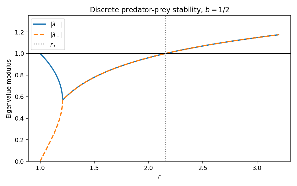
As $r\downarrow 1$, $n_c\to 0$, so the roots approach one and zero. The characteristic polynomial at one is $n_c(1-b/r)>0$, putting the larger real root just below one and the other positive root below it. No real root can ever equal one. Moreoversince its numerator exceeds $r-1-\log r>0$. At $n_c=1$, $\tau =1+b/r<2$, so the roots are conjugate and nonreal. Just above this point their modulus is $\sqrt{n_c}>1$.

The unit-disc conditions are $1-n_c>0$, $1-\tau +n_c>0$, and $1+\tau +n_c>0$. The last two hold automatically here, so stability is equivalent to $n_c<1$. The unique crossing and its eigenvalue argument satisfyIndeed $\log r_{\ast }=1-b/r_{\ast }<1$. This is the stability threshold of a discrete exponential predator-prey model. The sketch uses $b=1/2$: the real moduli merge and then coincide, increasing through one at the threshold. Linearization decides stability below and instability above; it does not determine nonlinear stability exactly at the crossing.

A horseshoe for an interval map consists of an open interval $J$ containing two disjoint open subintervals each mapped onto $J$. Glendinning chaos means that some positive iterate has a horseshoe.

Solving on the appropriate branches of the tent map givesHere $F(x_{-2})=x_{-1}$ and $F(x_{-1})=x_0$. On $J=[x_{-1},x_0]$ the second iterate isBoth endpoints map to $x_0$, and the minimum is $v=\mu -{\mu }^2/2$. Both monotone branches cover $J$ when $v\le x_{-1}$, equivalently $(\mu -1)({\mu }^2-2)\ge 0$. Restricting them to preimages of the interior proves a horseshoe for $F^2$ when $\mu \ge \sqrt{2}$.

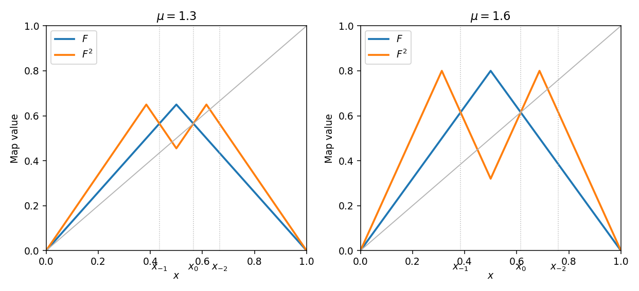
For $1<\mu \le \sqrt{2}$, $G(J)\subseteq J$. Set $d=(\mu -1)/(\mu +1)$ and $h(x)=(x_0-x)/d$. This maps $J$ onto $[0,1]$; substitution in each linear piece gives $hG{h}^{-1}=F_{{\mu }^2}$. The renormalization of the tent map near its fixed point therefore makes $F^4$ conjugate on $J$ to $F_{{\mu }^2}^2$. Applying the preceding threshold proves its horseshoe when $2^{1/4}\le \mu <\sqrt{2}$.

For $\mu \ge \sqrt{2}$, the inverse branch of $G$ fixing $x_0$ contracts distance to $x_0$ by ${\mu }^{-2}$. Compose $m$ copies of it with the other inverse branch. This contraction has a fixed point with a periodic itinerary, distinct from $x_0$ and at distance $O({\mu }^{-2m})$. Hence nontrivial periodic points accumulate at $x_0$.

For $\mu <\sqrt{2}$, the conjugate tent parameter $\nu ={\mu }^2<2$ has every nonzero periodic point in $[\nu -{\nu }^2/2,\nu /2]$. This interval is forward invariant; below it, a nonzero point increases until entering it. The positive lower bound separates those periodic points from zero, which corresponds to $x_0$. Thus no nontrivial periodic points are sufficiently close to $x_0$ from the left. A point sufficiently close on the right maps to such a left-hand point; periodicity would pass to its image and is impossible. Thus $x_0$ is isolated among periodic points, even though a fourth-iterate horseshoe exists elsewhere.

Differentiate $E=\rho c^2{a}^3{V}_0$ and use $dE=-PdV$, with $V=a^3{V}_0$. Division by $c^2{a}^3{V}_0$ givesThis is homogeneous adiabatic expansion without entropy production or exchange across the comoving element.

The two scalings give $\rho ={\rho }_{r0}{a}^{-4}+{\rho }_{s0}{a}^{-2}$. Flatness and the Friedmann equation give $H^2=8\pi G\rho /3$, with $H_0^2=(8\pi G/3)({\rho }_{r0}+{\rho }_{s0})$. ThusOn the expanding branch, putting the Big Bang at zero, separation givesIts positive square root is the required solution. If $\beta >0$, its early behaviour is $a\propto t^{1/2}$, as for radiation. The values $a=1$ and $a^2=\beta$ giveFor $\beta =0$ there is only the string component, with linear expansion and no radiation era.

For radiation $P_r/c^2={\rho }_r/3$, so $d\log {\rho }_r=-4d\log a$. Normalization at $a=1$ gives ${\rho }_r={\rho }_{r0}{a}^{-4}$.

For strings $P_s/c^2=-{\rho }_s/3$, so $d\log {\rho }_s=-2d\log a$. Thus ${\rho }_s={\rho }_{s0}{a}^{-2}$. These separate scalings assume no energy transfer between components.

True. For $\beta >0$, multiplication $\gamma \mapsto \beta \gamma$ is strictly increasing and continuous at limit ordinals, and $\beta \gamma \ge \gamma$. Thus there is a greatest $\gamma$ with $\beta \gamma \le \alpha$: the set is bounded, and its supremum still satisfies the inequality by continuity if it is a limit. The remaining ordered interval in $\alpha$ has an ordinal order type $\delta$, so $\alpha =\beta \gamma +\delta$. If $\delta \ge \beta$, then $\beta (\gamma +1)\le \alpha$, contradicting maximality. Hence $\delta <\beta$.

False. Take $\alpha =\omega +1$, $\beta =2$. For finite $\gamma$, $\gamma \cdot 2+\delta$ with $\delta <2$ is finite. For infinite $\gamma$, $\gamma \ge \omega$ implies $\gamma \cdot 2\ge \omega \cdot 2>\omega +1$. Neither case gives the required expression.

True. This is left distributivity of ordinal multiplication. Fix $\alpha ,\beta$ and induct on $\gamma$. The zero case is immediate. The successor step uses $\alpha (\eta +1)=\alpha \eta +\alpha$ and associativity of ordinal addition. At a limit, multiplication and addition are continuous in their right argument, so taking suprema of the earlier equalities gives $\alpha (\beta +\gamma )=\alpha \beta +\alpha \gamma$.

False. For $\alpha =\beta =1$ and $\gamma =\omega$, the left side is $2\cdot \omega =\omega$, whereas the right side is $\omega +\omega >\omega$.

Under the convention that a limit ordinal is nonzero and not a successor, the assertion is false at $\alpha =0$, since $\omega \cdot 0=0$. It is true for $\alpha >0$. If $\alpha =\eta +1$, then $\omega \alpha =\omega \eta +\omega$ has no greatest predecessor. If $\alpha$ is a nonzero limit, $\omega \alpha ={\sup }_{\eta <\alpha }\omega \eta$, again a nonzero limit. If zero is counted as a limit ordinal by convention, the unrestricted assertion is true with that convention.

True. Divide a limit ordinal $\lambda$ by $\omega$ using part a: $\lambda =\omega \alpha +n$ with $n<\omega$. If $n>0$, the right side is a successor, contrary to the limit assumption. Hence $n=0$ and $\lambda =\omega \alpha$. For a nonzero limit, $\alpha >0$; if zero is allowed as a limit, it is represented by $\alpha =0$.

Work with finite graphs, as in the usual matching theorem. Hall's condition is $|N(A)|\ge |A|$ for every $A\subseteq X$. It is necessary because a matching injects $A$ into its neighbours.

For sufficiency, induct on $|X|$. If a nonempty proper subset $A$ has $|N(A)|=|A|$, induction matches $A$ to $N(A)$. For $B\subseteq X\setminus A$, Hall's inequality for $A\cup B$ gives $|N(B)\setminus N(A)|\ge |B|$, so induction matches the complement to unused neighbours. Combining the matchings finishes this case. Otherwise every nonempty proper $A$ has $|N(A)|\ge |A|+1$. Choose an edge $xy$, delete its endpoints, and observe that every subset of the remaining $X$ still has at least its own number of neighbours. Induction matches the remainder, and adjoining $xy$ finishes. The one-vertex case and the empty case are immediate.

For $0\le d\le |X|$, the defect version isNecessity follows because at most $d$ vertices of $X$ can be unmatched. For sufficiency add $d$ new vertices to $Y$, each joined to every vertex of $X$. The displayed inequality makes Hall's condition hold in the enlarged graph. Its full matching uses at most $d$ new vertices, giving the required original edges.

To prove the matching-cover equality, let $M$ be a maximum matching and $U$ its unmatched vertices in $X$. Follow alternating paths from $U$, using nonmatching edges from $X$ to $Y$ and matching edges back. Let $Z_X,Z_Y$ be the reachable sets. No reachable $Y$ is unmatched, since that would give an augmenting path and a larger matching. Matching edges give a bijection $Z_Y\leftrightarrow Z_X\setminus U$. The set $C=(X\setminus Z_X)\cup Z_Y$ covers every edge: an edge from a reachable $X$ to an unreachable $Y$ cannot be a nonmatching edge, and its matching edge, if present, is already reachable. Its size isEvery vertex cover has at least $|M|$ vertices, because the matching edges are disjoint. Therefore maximum matching size equals minimum vertex-cover size, as required.

Begin with two points at distance one. A ruler draws the line through two known points; a compass draws a circle with a known centre and a constructible radius. New points are intersections of such lines and circles. A real number is constructible when it occurs as a coordinate of a point obtained by finitely many such operations; a complex point is constructible when both coordinates are.

If current coordinates lie in a field $K\subseteq \mathbb{R}$, a line-line intersection solves linear equations over $K$, while line-circle or circle-circle intersections reduce to a quadratic equation over $K$. Thus each step requires at most adjoining a square root. Consequently every constructible number lies in a towerConversely field sums and differences are obtained by laying off segments, products and quotients by similar triangles, and a positive square root by the geometric-mean construction in a semicircle. Hence every real number in such a tower is constructible. This proves the quadratic-tower criterion, not merely its necessity.

In particular a constructible algebraic number has degree a power of two. Degree alone is not sufficient in general; the exact criterion is containment in a quadratic tower. Equivalently the Galois group of its normal closure is a finite two-group: a tower's normal closure remains a two-extension, and a two-group admits a chain of subgroups with successive index two, yielding the converse by Galois correspondence.

The standard impossibility results follow. Doubling a unit-volume cube requires $\sqrt[3]{2}$, whose polynomial $X^3-2$ is irreducible by Eisenstein and has degree three. Trisecting an arbitrary angle would in particular trisect $60$ degrees, requiring $2\cos 20^{\circ }$, a root of $X^3-3X-1$. This cubic has no rational root and is irreducible, so this construction is impossible, although some particular angles can be trisected. Squaring the unit circle requires side length $\sqrt{\pi }$, impossible because $\pi$ is transcendental whereas constructible numbers are algebraic.

For a regular $n$-gon, constructibility is equivalent to that of $e^{2\pi i/n}$. The cyclotomic extension is Galois of degree $\phi (n)$, so it is constructible exactly when this degree is a power of two. Writing the prime factorization of $n$ shows the equivalent conditionIndeed odd prime exponents must be one, and each $p_i-1$ must be a power of two. If $2^m+1$ is prime, $m$ must itself be a power of two by factoring when $m$ has an odd divisor. Conversely this factorization makes the cyclotomic Galois group a two-group and provides a quadratic tower. This gives both positive constructions, such as the regular seventeen-gon, and obstructions, such as the regular seven-gon.

The conjugacy classes are specified by cycle type, with sizes $1,6,3,8,6$ for $1,(12),(12)(34),(123),(1234)$. The trivial and sign representations give the first two rows. The permutation representation on four letters contains a trivial line; its orthogonal complement has character equal to the number of fixed letters minus one. Tensoring that representation by the sign gives another row. Finally the quotient $S_4/V_4\cong S_3$ supplies the two-dimensional standard representation. The resulting table isWith the class-size-weighted inner product, these characters have norm one and are pairwise orthogonal, so all are irreducible and inequivalent. Their squared dimensions sum to $1+1+9+9+4=24=|S_4|$, proving completeness.

The classes of $A_4$ are the identity, the three double transpositions, and two classes of four three-cycles. Its quotient by $V_4$ is cyclic of order three, giving characters $1,\chi ,{\chi }^2$, with $\chi$ taking values $1,1,\omega ,{\omega }^2$ on these classes. The restriction of $V$ has character $(3,-1,0,0)$ and norm $(9+3)/12=1$, so it is the three-dimensional irreducible representation $T$. These four representations are complete since $1+1+1+9=12$.