The Steinitz exchange lemma says that if span a vector space and are linearly independent, then , and after reordering the , the family still spans. Here is a proof. Suppose the first replacements have been made. Express in that spanning family. Some coefficient of a remaining must be nonzero, since otherwise belongs to the span of , contrary to linear independence. Solve for that and replace it by ; this preserves spanning. If , the first replacements leave a spanning family , contradicting linear independence of the first vectors. This proves both assertions.
Now suppose is linearly independent and spans . Express each member of the standard basis using finitely many members of , and let be the finite union of those members. Then spans. No element of can exist, since it would be a linear combination of and violate linear independence. Thus is finite. Applying the Steinitz exchange lemma in both directions to and the standard basis gives and . Hence .
If is linearly independent and has elements, apply the Steinitz exchange lemma with as the independent family and the standard basis as the spanning family. All members of the standard basis are replaced, leaving itself spanning. Thus , so is a basis.
If spans and has elements but is linearly dependent, a nontrivial linear combination equal to zero lets us remove one member without changing the span. This produces spanning vectors, whereas the standard basis contains linearly independent vectors, contradicting the Steinitz exchange lemma. Therefore . Together the three deductions establish that any two of the three properties imply the third. For , the only independent or zero-element family is the empty basis, and the same conclusions hold.
Relative to the given basis , the proposed vectors are the columns ofThe determinant is nonzero exactly when the columns form a basis. Thus . At the vectors coincide, and at they are negatives of one another.
For complex differentiability at a point, the derivative must have the same value along real and imaginary increments. Along real increments it equals , while along imaginary increments it equals . Equating real and imaginary parts gives the Cauchy-Riemann equationsFor the given real part,Integrating the Cauchy-Riemann equations gives a harmonic conjugateThis open set is open and connected; is holomorphic there with derivative . The origin must be excluded because the real part is undefined there. On this connected open set, any other harmonic conjugate differs by a real constant: the Cauchy-Riemann equations make both partial derivatives of the difference zero.
In the curvature normalization, the hyperbolic triangle area is its angle defect:Join one vertex of a convex geodesic polygon to its nonadjacent vertices. This gives hyperbolic triangles with disjoint interiors. Their angles at every polygon vertex sum to that vertex's interior angle. Adding the hyperbolic triangle areas therefore gives the hyperbolic polygon areaFor a regular hyperbolic polygon with prescribed area, place equally spaced vertices on a hyperbolic circle of radius and join consecutive vertices by geodesics. Rotations through and reflections in radial lines show that this is a convex regular polygon. The triangle from its centre to a vertex and the midpoint of an adjacent side is right angled, with angles , , and , and hypotenuse . The angle form of the hyperbolic law of cosines givesConsequently is continuous and strictly increasing. As , , so ; as , , so . The intermediate value theorem proves existence for every permitted . Indeed the required radius isThe argument also proves uniqueness of the radius in this construction; neither endpoint area is attained by a nondegenerate finite-radius polygon.
Take a smooth variation with on the boundary. Assume enough differentiability for the following operations, for example a smooth bounded open set, , and a twice continuously differentiable integrand. Differentiation under the integral givesBy integration by parts, the boundary term vanishes and the first variation isStationarity for every such variation, including every compactly supported smooth one, and the fundamental lemma of the calculus of variations give the Euler-Lagrange equationFor the quadratic integrand, , , and . Thuswith the prescribed Dirichlet boundary condition. For real , a stationary function is also the unique minimizer, if it exists: for any nonzero admissible , the linear term vanishes and . This last positivity uses the zero boundary values; it also holds at .
The divergence and scalar vorticity areThus the flow is irrotational but not incompressible on the plane. A velocity potential satisfying isIndeed its two partial derivatives are the two velocity components. A usual two-dimensional stream function would satisfy , and hence have identically zero divergence. No such stream function exists on an open region where this divergence is not identically zero; the line is not a two-dimensional flow domain.
Here both the divergence and vorticity vanish:The flow is incompressible and irrotational. With and ,The streamlines are the level sets . To determine the arrows, put and . A particle satisfies , . Thus the separatrix approaches the stagnation point at the origin, whereas leaves it; the other streamlines are hyperbolas following those asymptotes. The origin itself is a stationary particle.
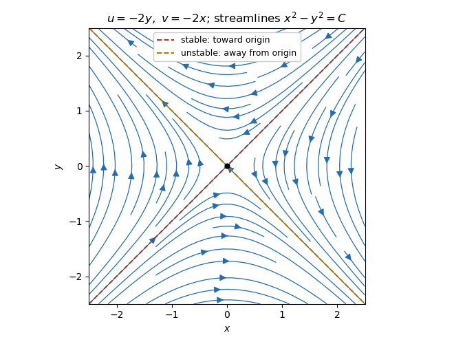
Streamlines and directions for the incompressible irrotational flow
. The Lagrange cardinal polynomials areThus the Lagrange interpolation polynomial isIt has degree at most and takes the required values. Uniqueness follows because the difference of two such polynomials has distinct roots and degree at most , so is zero. The source's phrase “degree ” must allow a smaller degree, for example when is constant.
Define the divided difference recursively by andInduction on this recursion, or comparison of the leading coefficient in the Newton interpolation polynomial, givesFor completeness the induction works term by term: an interior term gets the coefficient , multiplying the product over the other interior nodes; the two endpoint terms give the same formula. This is also the leading coefficient of directly from the cardinal formula, so .
The function has distinct zeros. Repeated application of Rolle theorem gives with when . HenceFor , this is simply and we take .
The Rao-Blackwell theorem applies to an estimator with finite second moment and a sufficient statistic . The conditional estimator can be chosen as a function of the observed that does not depend on the unknown parameter: this uses the parameter-independent conditional data distribution in the definition of sufficient statistic. The tower property of conditional expectation gives , so their bias agrees. The law of total variance givesFor any target it follows thatEquality holds exactly when almost surely under that parameter value. This proves variance reduction and reduction of mean squared error, whether or not the original estimator is an unbiased estimator. More generally, conditional Jensen inequality proves the corresponding inequality for any convex loss in the estimate, whenever the expectations exist.
Since , the indicator is an unbiased estimator of . The joint probability mass function isThe Fisher-Neyman factorization theorem therefore makes a sufficient statistic. More explicitly, conditioning on gives a multinomial distribution with trials and cell probabilities , so has the binomial distribution . Consequently conditioning by the Rao-Blackwell theorem givesFor , interpret the value at as and at as ; thus the same expression uses in this probability convention. For all observations and are zero almost surely. For and , the reduction in variance is strict: given , the event still has a nondegenerate conditional probability. Directly, using the probability generating function of , the new variance is .
Introduce nonnegative slack variables and use the origin as the initial feasible simplex basis:In the simplex method, let enter. The ratio test is , so leaves. Solving the first constraint for yields the dictionaryAll nonbasic variables are nonnegative and have negative reduced objective coefficients. Setting them to zero is feasible and optimal:Subtracting from both right-hand sides changes the same dictionary toIt remains feasible throughout , including the degenerate endpoint , and the reduced coefficients are unchanged. HenceAs an independent optimality certificate, , with equality at the stated point. Negative reduced coefficients also prove uniqueness of the optimal decision vector.
False. A left inverse would force to be injective: if , then . Take the surjective linear map given by . Since belongs to its kernel, every composite annihilates and cannot be the identity map on .
True. Choose a basis of . By surjective function, choose with . Define the linear map by and extend by linearity. Then on every basis vector, and thereforeThis constructs a right inverse and does not require to be injective. If is the zero vector space, the unique zero map is the required right inverse.
True. Use the lifted basis above and put . If , applying gives , so all . Thus the form a basis of , and takes this basis to the basis of . It is a linear isomorphism.
In fact the right inverse gives the stronger splittingFor every , write ; the first term is in the kernel and the second in . Their intersection is zero because is injective. This is a direct sum decomposition.
False. Take , , , , and . Then is a direct sum, but , so their intersection is not zero. Their ordinary sum is , as always follows from surjective function and ; the failure is precisely the direct sum assertion.
False. Take , , and . Then , but because is missing. Thus the premise does not force spanning. It need not force zero intersection either: with the same , take and . Their images still have a direct sum, while .
The Sylow theorems state that if a finite group has order with prime and , it has a subgroup of order , called a Sylow subgroup. Every p-group subgroup is contained in a Sylow subgroup, and all Sylow subgroups for the same prime are conjugate subgroups. Their number satisfiesMore precisely for a Sylow subgroup , where is its normalizer.
A finite nonabelian simple group cannot be a p-group: a nontrivial finite p-group has nontrivial centre of a group, since its class equation makes every noncentral conjugacy class size divisible by , and hence makes the centre size a positive multiple of . That centre is a normal subgroup, so must be the whole group if is a simple group, making it abelian; an abelian simple group has prime order. Therefore every Sylow subgroup here is nontrivial and proper. It cannot be normal, so .
To obtain a simple group embedding from Sylow conjugation, the conjugation action on Sylow subgroups gives a group homomorphism . This group action is transitive by the Sylow theorems and is nontrivial since . Its kernel of a group homomorphism is a normal subgroup, so the defining property of a simple group makes the kernel of a group homomorphism trivial: is an embedding. Now compose with the sign of a permutation . A nontrivial composite would again be injective because is a simple group, embedding in a group of order two, impossible for a nonabelian group. Thus lies in the alternating group . By Lagrange's theorem,The argument only invokes the factorial formula once ; the impossible case itself is also excluded by the embedding.
For order , the Sylow theorems give and , hence or . If , the Sylow subgroup of order is a nontrivial proper normal subgroup. If were simple in the other case, it would be nonabelian (a finite abelian simple group has prime order), and the preceding result would force , impossible. Thus every group of order 48 is not simple.
An example with no normal Sylow subgroup for isIn , is a dihedral group of order : conjugation by inverts . Thus has order and is a Sylow subgroup of . The only transpositions in are and ; conjugating by gives . Therefore and are not normal. By conjugacy, no other Sylow subgroup for is normal either.
A real function on a metric space is uniformly continuous if for every there is a such that, simultaneously for all , implies . For a continuous function on a finite closed interval , suppose this fails. Then there are and pairs with but . By compactness, some subsequence converges to ; then too. Continuity contradicts the image separation. This proves the Heine-Cantor theorem in this setting. Boundedness of the interval matters: on is a counterexample if “closed interval” includes unbounded intervals.
A function is Lipschitz continuous if some finite satisfies for every pair. Choosing proves uniform continuity.
The first assertion is false. Take , which is bounded and continuous, andThen , , while . This violates uniform continuity.
True. If everywhere, the mean value theorem applied between any two distinct points givesThus is Lipschitz continuous and hence uniformly continuous. No continuity of is needed: differentiability of gives continuity on each finite closed interval and is exactly the hypothesis needed for the mean value theorem there.
True. Define and . The map is Lipschitz continuous with constant one. The restriction of to is uniformly continuous by the Heine-Cantor theorem; its modulus of continuity combined with proves uniform continuity of on all of . For each fixed , once we have . HenceThis pointwise approximation by uniformly continuous functions even gives eventual equality on every fixed bounded interval. It need not give uniform convergence on the whole line, as the bounded counterexample in part (i) already demonstrates.
If a nonempty subset is not an interval, there are and with . The disjoint nonempty relatively open sets and form a separation, so is not connected.
Conversely, suppose an interval had a separation into relatively open nonempty sets . Choose , interchanging the names if necessary so . Put . Because contains a relative neighbourhood of , ; because contains a relative neighbourhood of , . Also . If , relative openness supplies points of just above , contradicting the supremum. If , a relative neighbourhood of excludes points of approaching from below, again contradicting the supremum. Thus every interval is connected, including a singleton and unbounded or open intervals.
TakeIt is closed, because its only accumulation point is and that point is included, and bounded. The Heine-Borel theorem makes it compact. The connected components of its complement are preciselyEach is an interval and therefore connected; none can be enlarged inside the complement across one of the intervening points of .
Let . If , use the constant path. Otherwise consider the countably many lines through and a point of , and through and a point of . Choose a line whose direction is not parallel to any of these lines; such a direction exists because there are uncountably many directions but only a countable set of forbidden ones. Every forbidden line meets in at most one point. Choose outside those countably many intersections and outside .
Neither segment nor meets : a forbidden point on either segment would put on the corresponding forbidden line. The piecewise linear pathlies in the complement. This proves that the plane minus a countable set is path connected.
If a homeomorphism existed, its restriction after removing a point would give a homeomorphism between and . The first is a path-connected space and therefore connected; the second consists of two separated intervals. Since homeomorphisms preserve connectedness, .
Fix . Truncate at and close it with the upper semicircle centred at , oriented counterclockwise. For large the only pole of the integrand inside is . Uniformly on the arc, is comparable to and , so the arc integral is and tends to zero. The line integral is absolutely convergent at infinity for the same decay reason. The Cauchy integral formula givesThe right-hand side is holomorphic on this open half-plane by the hypothesis, proving the required holomorphic function. The contour never passes through because its imaginary part is strictly above the line.
Write . For and , close upwards as before. The residue theorem includes the poles at and , and the assumed decay in the upper region makes the arc contribution vanish. ThusIt is essential to include the apparently exceptional point . The Laurent series there is with holomorphic. At that point the integrand is , whose residue is . HenceThe displayed difference is interpreted by its removable singularity. It therefore defines a holomorphic function at every point of the required half-plane, including .
For , close upwards. The pole at is outside this contour, while is inside; the pole is also outside. The residue theorem and the minus sign in the definition of giveThis rational function is holomorphic throughout , since its only pole lies above . In particular the formula includes : the original line-integrand has no singularity on there, and no evaluation of is needed. Closing downwards would require a decay hypothesis in the lower half-plane that has not been given; closing upwards avoids that unjustified step.
In the open strip , neither pole of is present. The two evaluations therefore giveBoth summands are holomorphic on this strip. This is a half-plane decomposition by Cauchy integrals; the pole subtraction in is what makes its extension holomorphic even at the upper pole of .
Use the Fourier transform convention , with inverse . Splitting at the origin, with to ensure convergence, givesThus
The original PDF has forcing ; the supplied TeX loses the absolute-value bars. Set . First assume and . The Fourier transform of a derivative, obtained by integration by parts with the boundary terms zero, is . Applying it and the preceding transform givesUsing the inverse Fourier transform pairs from part (i),Both decay conditions hold. The first derivatives of the two exponential terms cancel at zero, so is continuously differentiable there; the second derivatives have matching limits and the differential equation holds at zero as well as on both half-lines. For uniqueness, a difference solves the homogeneous equation. Decay gives on the positive half-line and on the negative half-line. Continuity gives and derivative continuity gives , forcing both to be zero.
The PDF's condition also allows , but no decaying solution exists when . Indeed on , and decay forces ; on , decay forces . Their one-sided derivatives at zero are and , which cannot match. The missing condition is therefore a genuine source omission, not a transcription repair. The transform expression at has a nonintegrable singularity, consistently with this obstruction.
For smooth rapidly decaying initial data, apply the Fourier transform in and differentiate under the integral. The Fourier transform of a derivative turns the wave equation intoSolving this constant-coefficient ordinary differential equation givesAt the quotient means its continuous limit , so .
Since , the Translation property of the Fourier transform inverts the first term as . Also has Fourier transform , including its limiting value at zero. The convolution theorem therefore inverts the second term asThis proves the D'Alembert formulaThe formula itself extends beyond the rapidly decaying class: and suffice for a classical solution, verified by differentiation and the two initial conditions. The decay assumption above justifies the ordinary transform derivation without distributional qualifications.
Define the parity operator by . For the usual full-line Hamiltonian operator, or any parity-invariant operator domain and boundary conditions, an even potential gives : the second derivative is unchanged by reflection and . If , then . A nondegenerate energy eigenvalue has a one-dimensional eigenspace, so for some scalar . Since , . HenceThus the stationary state has even or odd parity. The symmetry must include the operator domain: an even potential alone would not imply this conclusion with asymmetric boundary conditions.
A bound state has and , since outside the delta potentials a square-integrable solution must decay exponentially. The wavefunction is continuous at each delta: a jump would produce a delta derivative in with no matching term in the equation. Integrating the Time-independent Schrodinger equation across either givesThe symmetry of the symmetric double-delta potential permits even and odd solutions. Up to a nonzero normalization factor, the even candidate is for , and outside. Its derivative jump at givesThe odd candidate is inside and outside. Its jump givesParity ensures the jump at as well. Put and . The continuous strictly increasing function ranges from to infinity, so there is exactly one even bound state for every . The continuous strictly increasing function ranges from to infinity, so the odd bound state of a symmetric double-delta potential exists if and only if . Strict increase follows from the allowed monotonicity facts plus the strictly increasing term . ThereforeAt equality the odd limiting solution has and is not square integrable, so it is not a bound state. No nonnegative energy can supply another full-line square-integrable state, since its exterior solutions are oscillatory or affine.
In a source-free vacuum, Maxwell equations areTaking a curl of the last two equations and using gives the electromagnetic wave equationsSubstitution of the complex plane wave amplitudes into Maxwell equations, then taking real parts, givesFor a nonzero propagating wave these imply the dispersion relation . Conversely choose any nonzero transverse complex and set to obtain such a wave. The static uniform-field sector at is separate from propagation.
At a perfect conductor, the oscillatory boundary conditions are and . Surface charge and surface current allow nonzero normal electric and tangential magnetic fields. The magnetic condition here concerns the time-dependent wave field; a perfect conductor can retain a pre-existing static magnetic field.
Let be the orthogonal reflection across the boundary plane, so . The proposed reflected amplitudes are , , and . For an orthogonal reflection, . HenceAlso , so the reflected wave obeys the same dispersion relation. At , the incident and reflected phases coincide because is parallel to . Their summed amplitudes satisfyThe first has zero tangential part and the second zero normal part, proving both boundary conditions. Finally , as required for reflection into the vacuum.
Choose downslope along the rigid plane and normal to it into the fluid, with the wall at and the flat free surface at . The gravitational body force per unit volume has components . The wind's tangential traction on the top surface is in the direction; the atmospheric normal traction is in the direction. At the wall there is no-slip boundary condition, and the wall supplies the opposing normal force and a tangential traction whose sign depends on the wind strength.
The velocity is parallel to the plane, . Its velocity profile is a concave quadratic, with and negative slope at the free surface when . The diagram uses moderate wind, for which the flow is still everywhere downslope. Stronger wind can reverse the upper portion, or the entire moving layer; the later cases quantify this.
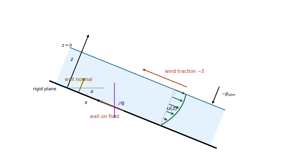
For an inclined viscous film with opposing surface shear, the steady parallel velocity automatically satisfies the continuity equation and the advective acceleration vanishes. The two components of the Navier-Stokes equations reduce toThe uniform thickness and constant atmospheric pressure make . The boundary conditions areThese are respectively no-slip boundary condition, imposed tangential traction on the surface with outward normal , and the normal stress condition on the flat free surface. The normal viscous stress is zero because the normal velocity vanishes. Integrating givesIn particular is the downslope tangential traction exerted by the fluid on the wall. The wall's tangential traction on the fluid has the opposite sign, because the outward normal of the fluid at its bottom is . This fixes the potentially confusing wall sign convention.
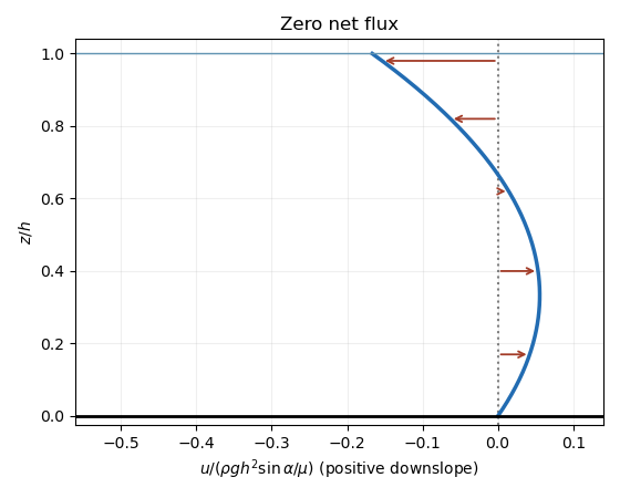
The volume flux per unit transverse width isThusAssume a genuinely inclined plane, . With and , the zero-flux velocity profile is . It is positive for , zero at , and negative above that level. Its maximum is at , and its surface value is . Thus equal integrated downslope and upslope transports cancel, rather than the fluid being motionless.
The wall shear stress vanishes when . ThereforeFor a genuinely inclined plane the entire moving layer now flows upslope. The profile touches zero at the wall with zero derivative and becomes increasingly negative towards the surface. In the plot with velocity horizontal and height vertical, the zero derivative at the wall is represented by a vertical tangent. The resulting volume flux is , so zero wall shear stress does not mean zero flux.
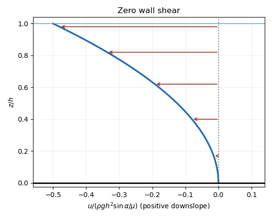
Zero wall shear and an entirely upslope velocity profile
. Assume is sufficiently smooth, for example near the exact trajectory. Write at the current value, with a linear map and a bilinear map when the ordinary differential equation is vector valued. Taylor expansion of the stages givesThe exact flow has Taylor expansionMatching the terms through in the Runge-Kutta method gives the sufficient third-order conditions for an explicit Runge-Kutta methodFor scalar , replace by and by in the scalar sense. The resulting local error is ; under a local Lipschitz continuity assumption and bounded derivatives on a finite time interval, the standard one-step error recurrence gives global error , hence third order.
On the linear test equation , putting gives the stability functionThus , so lies inside the linear stability domain. The four order conditions are compatible, for example and .
A sufficient statistic has a conditional distribution of the full data given its value that is independent of the unknown parameter. A minimal sufficient statistic is sufficient and is a function of every other sufficient statistic, up to null sets. For a dominated family with common positive support, the likelihood-ratio criterion for minimal sufficiency states that is minimal sufficient if holds exactly when is independent of .
For , the joint probability mass function isThe Fisher-Neyman factorization theorem proves sufficiency of . For two samples, the likelihood ratio is , independent of exactly when their sums agree. Thus is minimal sufficient. Any one-to-one transformation of it is also minimal sufficient, so chooseThis chosen estimator is an unbiased estimator, since each observation has mean . If instead the statistic is reported as , its expectation is , and as an estimator of it has bias (zero only when ). Being a minimal sufficient statistic is unchanged by this rescaling; being an unbiased estimator is not.
For a target , the bias of an integrable estimator is ; it is an unbiased estimator if this is zero at every allowed parameter value. Here has a zero-truncated Poisson distribution, , and . Write an estimator based only on as , assuming a finite expectation for every . Unbiasedness requiresAbsolute integrability at every positive parameter ensures that the power series on the left converges absolutely on every complex disc. Uniqueness of coefficients in a power series therefore gives for odd and for positive even . Conversely these values give the displayed identity, sois the unique unbiased estimator of this form. The uniqueness claim concerns nonrandomized functions of ; allowing external randomness would permit addition of independent mean-zero noise.
For this parity estimator for a zero-truncated Poisson count, usefulness depends on the loss, but under squared-error loss it performs poorly despite being an unbiased estimator. Since , andIt takes the inadmissible value with positive probability, and its variance tends to one rather than zero as . Clipping to the parameter interval gives . This has bias , butThus a simple biased estimator strictly improves its mean squared error at every parameter value; uniqueness among unbiased estimators does not make it optimal for this loss.
Assume the intended initial fortune satisfies and put . Conditional on current fortune , the next gift is uniform on and independent of the previous choices. The remaining fortune is therefore uniform on that same set. At fortune the process stays there. Consequently the future conditional distribution depends only on the current fortune, proving the Markov property, and the transition matrix on isThe uniform decreasing Markov chain has state as an absorbing state, and until absorption the fortune strictly decreases, so the hitting time is at most .
Let be the expected number of additional transitions to hit , taking . First-step analysis givesIn particular . For , multiplying this recurrence by and the recurrence for by , then subtracting, gives . Hence for every , and telescoping yieldsThe PDF defines using times . If were included, that definition would give although the displayed empty sum is zero; the initial instruction to choose an integer between and also requires . The result above uses that intended assumption. A hitting time allowing time zero would have expectation zero from state , but that is a different definition.
Articles by others on the same topic
There are currently no matching articles.