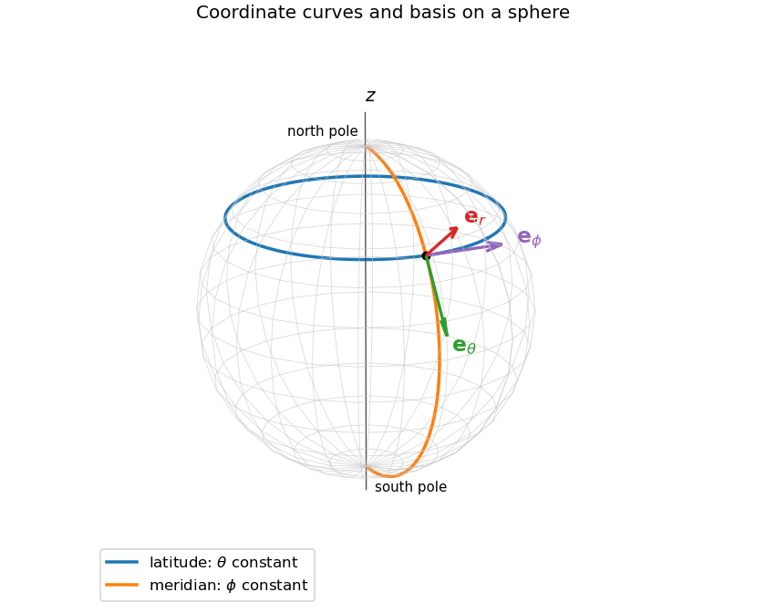
On the sphere, constant gives a latitude circle of radius and height . Constant gives a meridian semicircle in a vertical plane through the axis. The orthonormal basis of spherical coordinates isHere points outward, along increasing polar angle, and along increasing azimuth. At either pole the radial unit vector is unambiguous, but the two tangential coordinate vectors depend on the undefined longitude. The figure shows their directions away from the poles.
This coordinate ambiguity does not make a vector field singular if its tangential coefficient vanishes suitably. In Cartesian coordinates,The first is smooth at the north pole and zero there; the second is smooth and zero at the south pole. Their actual singular axes are the opposite ones. These are the regular patches of a two-patch vector potential for a radial monopole.
Along the circle with increasing , the line element is . Thus the two circulations areThe half-angle identities simplify them toHere so both potentials are defined on the whole curve.
For an axisymmetric azimuthal vector field, the curl in spherical coordinates has componentsThe angular expressions are and , each with derivative . Also is independent of , so the second component vanishes. Consequently, on each potential's regular patch,
The outward area element is . ThereforeSplit the sphere into the northern cap and the southern cap . Their induced boundary orientations are and , respectively. The Stokes theorem applies to on the north and on the south. Adding their fluxes gives , agreeing with direct integration.
There is no contradiction with the flux of a globally smooth curl through a closed surface: neither potential is regular on the entire sphere. On their overlap they differ by , a local gauge transformation. The longitude is not a globally single-valued scalar, so that difference can have nonzero circulation around .
Take a nonzero separated solution . Dividing by separates the Laplacian eigenfunction equation into and . The zero-endpoint Dirichlet boundary conditions admit no nonzero linear or hyperbolic factors, so both separation constants must be positive squares. HenceAll separated nonzero solutions have this form. At a repeated eigenvalue, linear combinations of the corresponding modes are also solutions, though they need not remain separable.
Multiply by the sine product and integrate over the square. Fourier orthogonality gives squared norm , and thusThereforeThis double Fourier sine series equals one at interior points. At boundary points every summand vanishes, consistent with the endpoint value of the sine extension.
Each spatial eigenfunction acquires the temporal factor under the heat equation. Expanding the initial constant using the preceding coefficients gives the cooling of an initially uniform square:For the exponential factors justify differentiating the series and enforce the zero boundary temperature. As , it tends to at every interior point and in L2 space; the instantaneous boundary cooling is incompatible with continuity at the initial boundary corners, which is expected for this idealization.
The slowest decaying nonzero mode is , givingat each fixed interior point when . The next contributing modes have and decay as , making the leading-mode approximation exponentially accurate.
Let . A Green's function satisfies and the chosen homogeneous boundary conditions in . Away from , it is a linear combination of and . It must be continuous there and obey the unit derivative jump , because the leading differential coefficient is one. Thensolves whenever the integral and boundary limits are valid. The Wronskian of is . The Green kernels for a radial dipole Euler equation implement the two different choices of boundary conditions below.
The factor satisfying the left condition is , while satisfies decay at infinity. Matching the value and unit derivative jump givesFor the specified compactly supported forcing, integrating over givesFor example, on , the two pieces contribute and . Both and match at one, and the function tends to zero at both ends. A homogeneous difference with those two limits must vanish, establishing uniqueness.
The zero initial value and slope select a forward Green's function: set it to zero for , and choose the right piece to start at zero with slope one. This givesFor on and zero elsewhere,Indeed . It and its first derivative match at one, while at zero. The only homogeneous solution with these two initial limits is zero, so this solution too is unique. Its growth at infinity is allowed by these boundary conditions.
Use the angular-frequency Fourier transform conventionFor the piecewise smooth functions here, the inverse gives the function at continuity points and the mean of one-sided limits at a jump. Values assigned at individual points do not affect the transform.
The even extension is the triangular function for and zero outside. Its Fourier transform is real and even:At zero the removable limiting value is one, also obtained directly by integrating the triangle. This is the Fourier transform of a triangular function.
For the odd extension, the cosine integral vanishes and the sine integral doubles. Integration by parts givesThe value at is zero by the odd function symmetry, or by the Maclaurin series of the sine. The transform is purely imaginary and odd.
For the chosen Fourier transform convention, Parseval's identity is . For smooth rapidly decaying functions its bilinear form follows by inserting the inverse transform of into and interchanging the integrals:Take . Approximation by such functions extends the identity to L2 space, which includes the compact triangular function here.
For that triangle, , while . ThusgivingThe continuous limiting integrand at zero is one. This is the sinc fourth-power integral.
A complex matrix is diagonalizable exactly when it has a basis of three linearly independent eigenvectors. If all its eigenvalues are one, a diagonalization would have and hence . Therefore the specified matrix, which is not a scalar identity matrix, is not diagonalizable.
For the displayed real symmetric matrix, choose the orthogonal matrixIts columns form an orthonormal eigenbasis, andIn the orthogonal coordinates , , the quadric surface has equation . It is a prolate spheroid, with long semiaxis one in direction and two equal short semiaxes . The figure gives its principal-axis sketch.
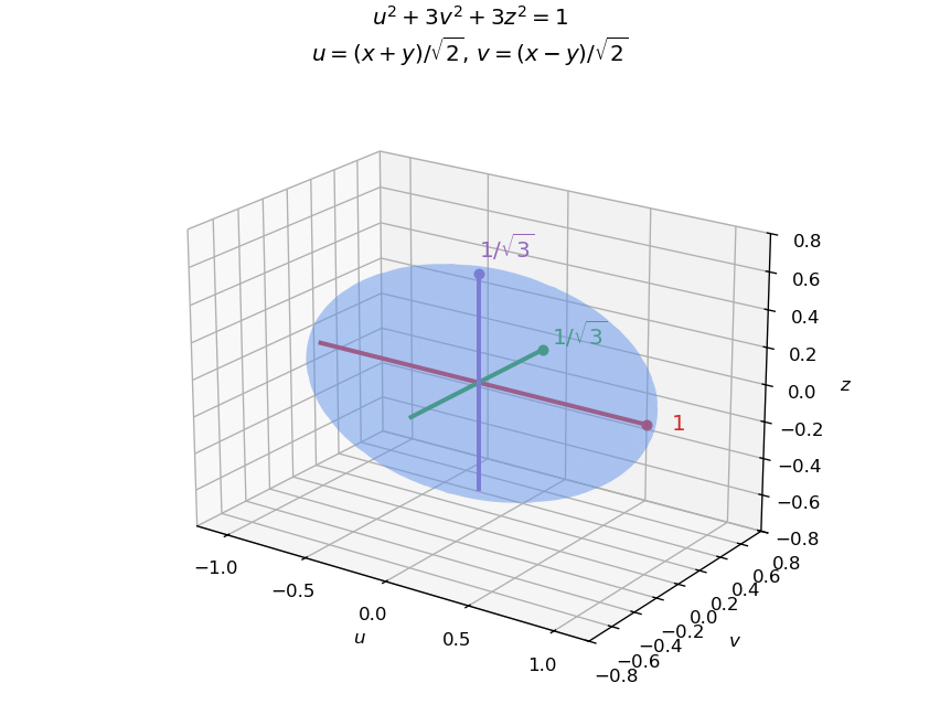
The diagonalized quadric is a prolate spheroid with semiaxes one and one over the square root of three
. Details. A diagonalizable matrix can certainly have exactly two distinct eigenvalues: is already diagonal and has an eigenbasis despite its repeated eigenvalue.
A Hermitian matrix satisfies . If with , then is real because its conjugate equals . Since , its eigenvalue is real. If with , thenso : distinct eigenspaces are orthogonal for the standard complex inner product.
The converse is false. For example has the two real eigenvalues one and two but is not a Hermitian matrix. It can be embedded as a block in a example if desired.
For Hermitian , . Thus is Hermitian exactly when , equivalently when their commutator vanishes. Also , so a value that works for every such pair isThis sum is their anticommutator.
For holomorphic in , the Cauchy-Riemann equations are and . Therefore the normal vectors to the two level curves obeyAt a point where , both gradients are nonzero, so their perpendicular tangent lines are also perpendicular. At critical points this argument does not assert that regular level curves exist.
TakeIts real part is , so the specified first family is . Its imaginary part is , so the second family is . Since , their intersections exclude the origin, where would vanish. Thus these hyperbolas meet orthogonally as required.
For an isolated pole of order , the Laurent coefficients must satisfyThen the principal part of a Laurent series is a finite sum with lowest power . The classification at the center assumes analyticity on a punctured neighborhood , or an analytic continuation there. A Laurent expansion on an annulus with positive inner radius alone does not imply that the center is an isolated singularity.
On a punctured neighborhood of the center, an essential singularity occurs exactly when infinitely many negative-power Laurent coefficients are nonzero. If all negative-power coefficients vanish, the singularity is removable; if finitely many are nonzero, the singularity is a pole. The punctured-neighborhood assumption matters: an annulus separated from its center cannot by itself classify the function there.
Put . Since and , the local Laurent series isThus all singular terms areThere is a third-order pole, with no second-order term.
Use the local coordinate at infinity. For positive integer ,The negative powers of this local coordinate are precisely . The singular part at infinity is thereforeInfinity is a pole at infinity of order . In the original variable these singular terms are positive powers; it is the negative powers of that define the local principal part of a Laurent series. For the point at infinity is regular, and for negative integer it is a zero rather than a pole.
The exponential power series gives for . Hence all singular terms areInfinitely many negative powers occur, so zero is an essential singularity.
Termwise differentiation of the convergent Frobenius series and collection of powers in the Bessel differential equation gives the lowest coefficient , the next coefficient , and, for , the coefficient . Since , the stated choices , and the recurrence make all coefficients vanish.
For , the two resulting even-coefficient series areandThese are linearly independent on and give the Bessel functions of order one half, up to normalization. The specified condition is sufficient; in the negative-exponent branch at this particular order the next coefficient equation alone would allow to be free, adding a multiple of the positive-exponent solution.
For the Legendre differential equation, substitution gives the full conditionsThus permits arbitrary , while requires . This Frobenius recurrence for the Legendre equation separates the even and odd series. The nearest singular points of the differential equation are , so the series about zero has radius at least one, and the generic nonterminating solutions have radius exactly one. Particular cancellations can give a larger radius.
Termination occurs when the degree reaches a nonnegative integer with . For this givesChoose the even branch for even or the odd branch for odd to obtain a Legendre polynomial. The recurrence then terminates and gives a solution for all real , with infinite radius of convergence. A nonzero entire solution at other is impossible: each nonterminating parity has coefficient ratio tending to one in the variable , and so radius one.
Take fixed-endpoint variations with . The first variation isThe boundary term vanishes by the endpoint conditions. The fundamental lemma of the calculus of variations gives the Euler-Lagrange equation . Along its solutions,When , this proves the Beltrami identity .
For the surface , the line element is . The arc-length integrand for a graph is . It has no explicit dependence and satisfies . Thus is constant. Choosing the fixed direction along a smooth nonconstant segment and integrating yieldsThe same result follows by defining the transverse arc coordinate , which changes the metric to . Its geodesics are straight lines in coordinates. This proves the formula for geodesics on a generalized cylinder and shows it gives locally shortest paths. The additional straight lines in the unrolled plane are also geodesics, but cannot be represented as graphs . Classical differential-geometric statements assume the surface has sufficient smoothness; the arc-length coordinate itself only requires the displayed integral to be well defined.
For nonzero with , the first variation of the Rayleigh quotient under isChoose fixed admissible homogeneous boundary conditions that make the variation boundary term vanish, such as zero endpoint values or zero endpoint derivatives. Compactly supported then show that a stationary function satisfies the Sturm-Liouville equation with . Conversely an eigenfunction satisfying those admissible conditions makes the variation zero. Multiplying its differential equation by and integrating by parts givesso the stipulated energy boundary term yields . The displayed energy condition alone is not a full specification of the admissible variations; it must be paired with boundary conditions for this variational equivalence.
For the final Dirichlet problem take the trial function , with . ThenThe Rayleigh-Ritz variational principle makes this an upper bound for the lowest eigenvalue. It is strictly above the true value: equality would require itself to be a lowest eigenfunction, but cannot vanish throughout for a constant . ThereforeAlthough the weight vanishes at the left endpoint, it is positive in the interior and its weighted quadratic norm is positive for every nonzero admissible continuous function; this does not obstruct the stated Dirichlet variational comparison.
Use the weighted inner product with positive weight . For a self-adjoint operator and nonzero eigenfunction , self-adjointness gives . The positive norm therefore forces to be real. For two eigenfunctions of distinct eigenvalues, the same calculation gives , proving their orthogonality.
The Chebyshev differential equation takes the Sturm-Liouville formIts operator is , so as required. For , direct substitution gives . Comparing coefficients yieldsExplicitly, using ,The endpoints are singular because vanishes and diverges there. The polynomial solutions use the natural condition at each end; under these are the Neumann eigenfunctions of the Chebyshev differential operator, proportional to . They differ from the zero-value endpoint realization of the same differential expression.
Let be the -periodic ramp represented by on . The Fourier series of a periodic sawtooth givesBoth boundary data are multiples of this odd function, so their angular means and cosine coefficients vanish. Consequently . Put . Matching the sine coefficients at the two radii gives and . Solving this two-by-two linear system yieldsEquivalently, two-boundary annular harmonic interpolation expresses the same solution asEvery term is a harmonic function, and the radial factors enforce the specified boundary values. For a radius strictly between and , their geometric decay makes the series smooth. At the boundary discontinuity , the limiting Fourier value is the mean of the two one-sided values, zero. The boundary data are imposed away from that exceptional point, as stated.
Away from its source, a radial two-dimensional Green's function satisfies , so . The divergence theorem on a disk of radius around the source requires , hence and . Choosing the additive constant givesThe equality with the Dirac delta is distributional; away from the source the Laplacian vanishes.
For the wedge, use the finite image construction for a planar wedge. In complex coordinates , place three positive sources at and three negative sources at , . The positive source at is the actual charge. The five images are thereforeOn either grounded ray, reflection pairs each positive source with an equally distant negative source, so their logarithmic potentials cancel. All images lie outside the open physical wedge. Summing their contributions with coefficient gives the required potential. The figure shows the bisecting-source configuration.
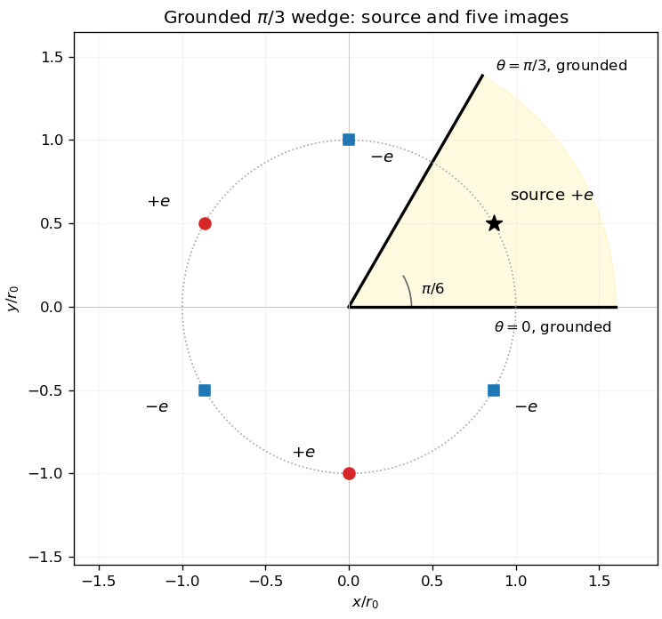


For , , the positive points are the three roots of and the negative points are the roots of . Thus the logarithmic sum isBoth boundaries have , verifying the zero potential directly. An arbitrary reference length inside the individual logarithms cancels because the six signed charges sum to zero.
For a simple pole, the residue is , the coefficient of its Laurent series. On an anticlockwise circle , integration of each Laurent term is zero except , whose integral is . This proves the stated single-pole residue theorem.
For , the only pole inside the rectangle of height is , with residue . The residue theorem therefore gives . The upper edge is traversed from right to left and satisfies , so the two horizontal contributions sum to .
On the right edge the modulus is bounded by , and on the left by . Multiplying by the fixed edge length shows that both contributions tend to zero because . ThusUsing yieldsThis rectangular contour for an exponential beta integral also gives the ordinary beta integral after the substitution .
Use . Jordan's lemma says that for , if a function has maximum modulus on upper semicircles, then ; a bound is . For use lower semicircles instead. The rational factors here meet this decay condition, so the residue theorem evaluates their inverse transforms.
For , only the upper half-plane contains a pole, at . Its residue after multiplication by is . The lower contour encloses no pole. ThereforeHere is the Heaviside step function, with midpoint value for symmetric Fourier inversion.
For , the upper-pole residue is when , while the clockwise lower contour gives the matching expression for . ThusThe final rational factor has double poles at . At the upper pole,The upper inverse integral is times that residue. The lower contour for negative supplies , and the value at zero is zero. Consequently
Under an orthogonal change of Cartesian coordinates with , a rank- Cartesian tensor transforms as , summing repeated indices. An isotropic tensor is invariant under every rotation. For an isotropic fourth-rank tensor, half-turns about the coordinate axes eliminate components unless each coordinate label occurs an even number of times. Coordinate rotations make the remaining two-pair patterns depend on three constants , , . Invariance after rotating the first axis to gives . HenceThis is a direct proof of the rank-four isotropic decomposition, without assuming any prior interchange symmetry of the four indices. Each displayed delta pairing is itself rotation invariant.
For symmetric strain, contraction gives . Comparing with the Lamé parameters yieldsWrite and , so . Since , the strain energy density becomesThe two terms describe volumetric and shear deformation, respectively. Thus nonnegative isotropic elastic strain energy is equivalent toNecessity also follows by taking a nonzero traceless strain and a pure dilation separately. The combination is the bulk modulus; strict inequalities give positive energy for every nonzero strain.
With downward position as the vertical coordinate, the full potential energy isThe equilibrium tensions are , and . On expanding, these relations cancel every term linear in the displacements, leaving . Newton's second law therefore givesFor a normal mode , set . The generalized eigenvalue problem isIts determinant is , so the angular frequencies and mode directions areThe square roots of these positive values give the requested frequencies. Only the lowest mode has all components of the same sign, so all three particles oscillate in phase at the lowest frequency. The mode shapes are shown below.
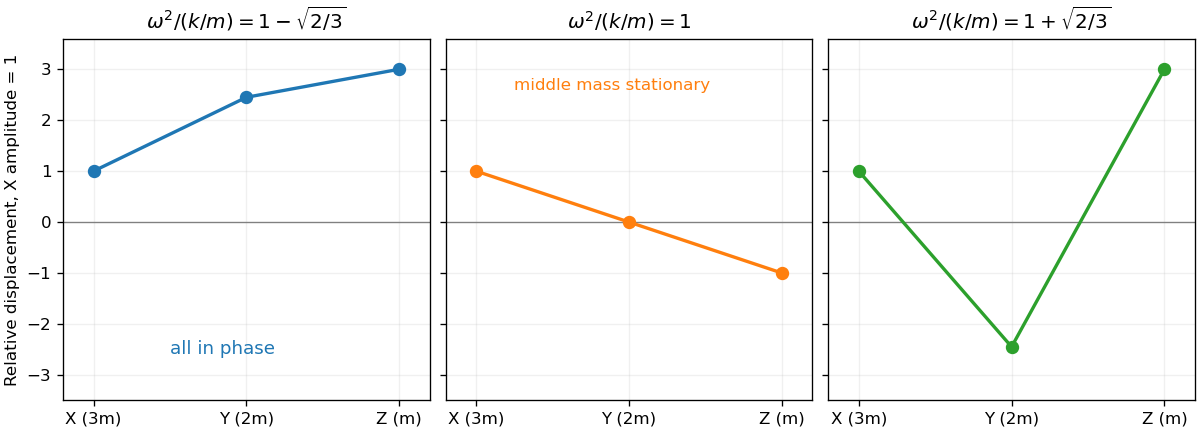
The three relative displacement patterns of the unequal-mass chain, from lowest to highest frequency
. Details. 
For release from rest with remaining at equilibrium, chooseThis excites only the middle-frequency mode, so for all time. It is a stationary middle mass in a three-mass spring chain: the equal and opposite adjacent spring forces cancel on .
If , then for both cosets equal . For , neither coset intersects : an intersection would imply . Both have elements, because multiplication by is a bijection. They therefore both equal , proving in this case too. This establishes that an index-two subgroup is normal.
For Lagrange's theorem, left cosets partition . Indeed if , then by multiplying by elements of ; otherwise the cosets are disjoint. Every coset has elements, so if there are cosets,The group order of thus divides the group order of . Normality is not needed for this divisibility statement.
The kernel of a group homomorphism is . It is a subgroup, since the identity maps to the identity and for . Alsoso . Applying the same inclusion with gives equality, proving that is a normal subgroup.
The map is well defined, multiplicative and injective, with image . Thus the first isomorphism theorem givesThe quotient is isomorphic to all of precisely when the original homomorphism is surjective.
For the general linear group, the determinant gives a homomorphism , since . Its kernel is the special linear group , so that subgroup is normal. Every nonzero real is the determinant of for , making the map surjective. Thereforewhere the operation on the right is multiplication.
Let . Since and , its powers define the representation of the cyclic group of order four:For the quaternion group, denote the three displayed complex matrices by . Direct multiplication gives , , , and . Together with the images of , these are exactly the quaternion multiplication relations, proving that the assignment defines a group homomorphism into .
Use the realification of a complex representation: for , define . It acts on grouped real and imaginary coordinates and satisfies . The explicit generators areSet and to specify all eight elements.
For an invertible real , the equivalent representation obeys . The trace is invariant under similarity, so their characters agree. Explicitly,
Articles by others on the same topic
There are currently no matching articles.