For a bounded volume with piecewise smooth closed boundary , and a continuously differentiable vector field on a neighbourhood of , the divergence theorem statesHere is the outward unit normal vector. The left side is the outward flux; the right side integrates the divergence over the enclosed volume.
The upper piece is a downward-opening circular elliptic paraboloid cap, running from the circle to the apex . The middle piece is the side of a circular cylinder of radius one and height one. The lower piece is the unit disk in the horizontal plane. Their union is the closed boundary ofThe four panels show the three separate pieces and their union; there is no additional fourth component. In a meridional section, the boundary consists of the base segment, two vertical sides, and the parabolic cap. The outward normals point downward on the base, radially outward on the cylindrical side, and upward/outward on the cap.
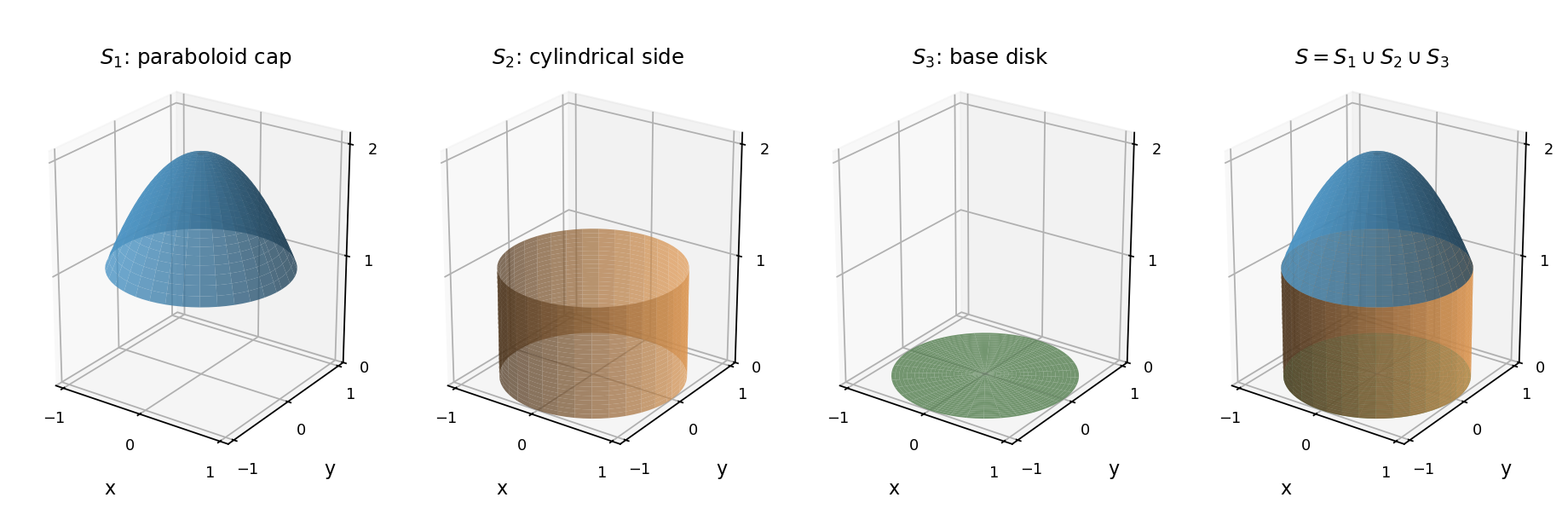
The polynomial vector field is smooth throughout the solid, so the divergence theorem applies. Differentiation givesThe volume is invariant under both and . Hence the integrals of the two odd terms vanish, and the flux is simply the volume. Using the circular cross-sections,The seams between the surface pieces have zero surface measure and contribute no extra term.
Set in the wave equation. A nonzero product obtained by separation of variables obeysThe fixed-end Dirichlet boundary conditions require . The zero and negative spatial eigenvalue cases produce only the trivial solution; the nontrivial eigenfunctions areFor each normal mode, . By superposition and completeness of the Fourier sine basis, the general finite-energy solution has the expansionIf and , orthogonality gives and . Individual products are separable; their sum is the general solution.
Assume the struck interval lies within the string, so . The initially stationary straight string has . Write its initial velocity as a Fourier sine series . ThenThus . Immediately after the strike all the energy is kinetic energy:The orthogonality integral assigns energy to mode . Since the ideal modes evolve independently, their total kinetic-plus-elastic energies remain constant. Therefore the modal energy of a localized velocity impulse on a string givesThe centre factor selects modes having significant motion at the impact location; the width factor accounts for cancellation across the finite hammer footprint. Parseval's identity ensures . The velocity discontinuities are understood in the mean-square sense and do not alter the energy integrals.
With the specified ratios, the two factors in the modal amplitude become and . Hence a normal mode is unexcited precisely when one of these factors is zero:That includes all multiples of five or fourteen, with multiples of seventy counted once. The mode is not a fixed-end string mode.
Away from , the homogeneous equation has solutions . A basis adapted to the two boundary conditions is at the origin and at infinity. Their Wronskian is . The Green function must be continuous at , while integration of across the source givesThese conditions give the Dirichlet half-line Green function for minus d2 plus 1:where and . The second term is the image that enforces ; both terms decay as .
For the finite forcing interval, . When , split the integral at :When , the entire source interval lies to the left, giving the Dirichlet half-line response to uniform interval forcingThis solution is unique: a homogeneous difference satisfying the origin condition is proportional to , which cannot decay at infinity unless its coefficient is zero.
The left-hand value at the junction isThe right-hand value isThus the piecewise Green function solution is continuous, withIts derivative is continuous as well: both one-sided values equal . Only the second derivative jumps, consistently with the step in the forcing and the absence of a Dirac delta source.
Use the Fourier transform conventionSince in distribution theory, the carrier has transformThe modulation property of the Fourier transform translates the message spectrum to the two carrier frequencies. ThereforeThe first term represents the unmodulated carrier wave; the other terms are the amplitude modulation sidebands.
A direct way to avoid the singular transform of is to invert a triangular function. Evenness givesAt the limit is , so there is no singularity in the original signal. ThusAlternatively, the hint uses the Hadamard finite-part reciprocal-power distribution, whose distributional Fourier transform is ; combining its three translates gives , the same triangle. Treating as an ordinary integrable function would be invalid.
The message spectrum has height at zero, vanishing at . For , the modulated continuous spectrum consists of disjoint triangles of height , centred at , each with half-width one. In addition there is a Dirac delta carrier line of weight at each centre. These lines have specified area, not a finite height; arrows mark them schematically.
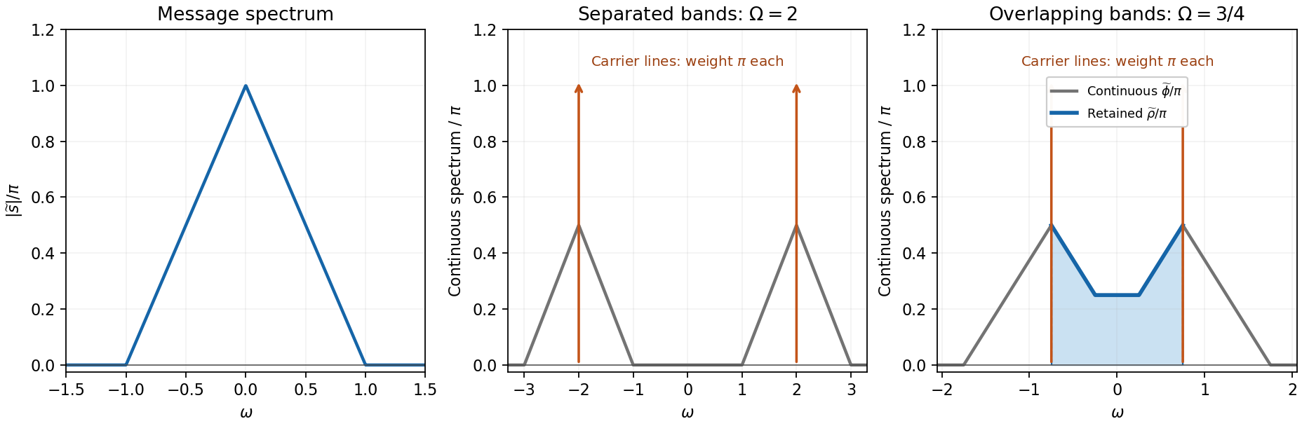
Triangular message spectrum, separated sidebands, and overlapping sidebands with the prescribed carrier-rejecting filter
. Details. At , the two continuous triangles overlap near zero. Their amplitudes add, giving a central plateau. Explicitly, write for the continuous part of :There are also the two carrier Dirac delta lines . The last panel of the preceding figure shows this spectrum and the retained central portion. The prescribed strict cutoff removes the carriers and keepsThe values of the ordinary function at individual endpoints do not affect its inverse transform. To handle the carrier lines, one must additionally assign zero filter gain to those lines, as the carrier-rejecting prescription indicates. A discontinuous mask has no canonical product with a Dirac delta at its discontinuity; a different physical boundary gain would leave a corresponding multiple of .
The retained spectrum is real and even. Its inverse Fourier transform isIntegrating the linear factors yieldsThe removable value is , obtained either by expansion or by integrating . Because the carrier frequency is below the message bandwidth, this is Fourier filtering of overlapping amplitude-modulation sidebands; the usual picture of two isolated bands in single-sideband modulation does not apply without that qualification.
The inverse is assumed to exist. First,By matrix commutation with an inverse, multiplying on both sides by givesAn equivalent calculation writes , so both products equal . No convergent infinite matrix series is needed.
Let be the real orthogonal matrix. If for a nonzero complex eigenvector, then preservation of the complex Euclidean norm givesso . Its characteristic polynomial has real coefficients, hence nonreal eigenvalues occur in conjugate pairs. Such a pair is , and the remaining real eigenvalue is or .
If all three eigenvalues are real, each is ; two have the same sign and can be paired as with or . Thus in every case the spectrum has the formTheir product shows that .
First, is invertible. If for a real vector, then , whereas the skew-symmetric matrix identity gives ; hence and . Thus its real kernel is trivial, which suffices for invertibility. The same argument applies to .
Using and the rule for the transpose of a product,The factors and commute, as do the required inverses. ConsequentlyThus . This is the Cayley transform of a real skew-symmetric matrix.
For a possibly complex eigenvector with , invertibility of gives . ThereforeThus every eigenvector of remains an eigenvector of . For a real skew-symmetric matrix, its eigenvalues have the form with real, so lies on the unit circle, consistently with orthogonality.
Taking determinants and using invariance under transpose,This determinant identity actually holds in every dimension. In dimension three, skew symmetry additionally givesso . Hence there is a real nonzero vector in the kernel:The eigenvalue relation then gives . Thus the Cayley transform fixes an axis and is a proper three-dimensional rotation, including the identity as a degenerate case.
A square matrix is diagonalizable over a specified scalar field if an invertible matrix exists such thatEquivalently, the underlying vector space has a basis of eigenvectors of : those basis vectors are the columns of , and their eigenvalues are the diagonal entries of . Here the field is unless specified otherwise.
Taking determinants of gives , so is singular and has the eigenvalue zero. More strongly, if with , then , so every eigenvalue is zero.
If the nilpotent matrix were diagonalizable, write . Then , hence each diagonal entry of has zero th power and is zero. Thus and . Conversely the zero matrix is diagonal. ThereforeThe conclusion is valid over and also over .
Use the full matrix in the original PDF; the transcription has dropped its middle column. For either matrix, the three-dimensional characteristic polynomial is . Both have zero trace and zero determinant, while and . ConsequentlyFor , a useful check isfor every value of . Thus is a nonzero nilpotent matrix for all ; for example its second column never vanishes. By the preceding result, .
For , the three eigenvalues are distinct and real, so their eigenvectors are linearly independent. An explicit eigenbasis isWith , and . Hence .
A repeated root of the characteristic polynomial alone would not settle diagonalizability; for it is the nonzero nilpotence that completes the argument.
A complex function is holomorphic at a point if it is complex differentiable throughout some open neighbourhood of that point. Writing and , a convenient sufficient and necessary criterion under continuously differentiable real components is the Cauchy-Riemann equationsThey must hold throughout an open neighbourhood, rather than at an isolated point. Merely having partial derivatives that satisfy these equalities at one point is not enough without an appropriate differentiability hypothesis. For the composition , holomorphy of and on the relevant open sets suffices; the additional condition is needed when using a local inverse conformal map, not for holomorphy of the composition itself.
Choose the branch of holomorphic in the upper half-plane whose boundary value at zero is . Thenand integration gives on this branch. The normalization and intended upper-half-plane image fix the otherwise ambiguous square-root sign.
To see the image, put . For and ,The bottom edge maps monotonically onto . The right wall maps by onto , and the left by onto . These boundaries describe the conformal map of a vertical half-strip by sine.
For completeness, the map is one-to-one in the interior: equality of two sine values forces arguments differing by or summing to , and neither alternative yields two distinct points in this half-strip. It is onto the upper half-plane as well. Setting gives ; the root product is , and no root lies on because that would make real. Thus exactly one root has . The identity then gives , so belongs to the half-strip. The closure gives the stated boundary-inclusive region; holomorphy is understood in its open interior.
In this region the transformed function is . Its only finite intrinsic branch point in the closure occurs where :It lies on the left boundary. There are no singularities in the open half-strip. The points , where diverges, map to the bottom corners; is holomorphic through those corners since there.
For the principal logarithm, the boundary segment , , is the preimage of its cut . Points on that cut above admit local analytic continuation after changing branch; itself is the genuine logarithmic branch point.
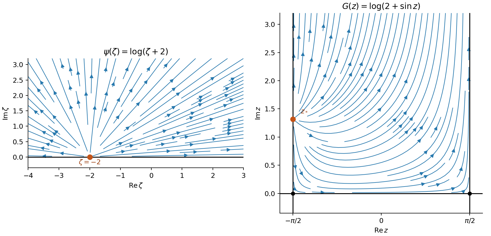
Writing ,ThereforeThe vector field points radially away from , with magnitude inversely proportional to distance from that point. It diverges on approach to that boundary point and tends to zero far away. This is the radial potential flow described by the logarithmic complex potential of a two-dimensional potential flow.
The chain rule givesTo make the directions explicit, set and . Multiplying by the complex conjugate of the denominator gives the logarithmic flow in a sine-mapped half-strip:In the open strip . The vertical component is negative near the lower left wall where , and positive above that curve. On the bottom the flow is rightward. On the right wall it is upward, whereas on the left wall it points downward below and upward above . The field is tangent to the boundaries except at the source and vanishes at the two bottom corners. At large , , so it tends to a uniform upward field .
Near , , showing a radial boundary source. The streamlines are the curves ; the figure shows their orientation without reusing the exam's graphics.


For the normalized second-order equation, is an ordinary point if both coefficient functions and are holomorphic near . If it is singular but and are holomorphic there, it is a regular singular point. Thus may have at most a simple pole and at most a double pole.
The distinction tells us which local series method is justified. At an ordinary point, two independent solutions are represented by ordinary Taylor series. At a regular singular point, the Frobenius method uses ; the indicial equation determines the exponents, and logarithmic terms may appear in a second solution. Singularities worse than these are irregular and need not have this Frobenius form.
The Wronskian isSuppose constants satisfy throughout the interval. Differentiating gives . At , these form the homogeneous linear systemIts determinant is nonzero by hypothesis, so . This is exactly linear independence of the two functions on the interval. No differential equation is needed for this implication; the converse for arbitrary differentiable functions would require additional hypotheses.
The origin is an ordinary point. Substitute into the equation and collect the coefficient of :Hence the recurrence relation isThere are two free initial coefficients. The independent even and odd power series beginThe general solution is . As a useful independent check, the substitution reduces the equation to . ThusFor a nonterminating parity series, , so the ratio test in gives . The regular singular points at explain the natural obstruction.
There is an important exception to an unconditional radius-one answer. If for an integer , the series of parity terminates at degree and is a multiple of a Chebyshev polynomial. Its radius of convergence is ; the other independent parity solution still has radius one. For the even solution is constant. Any nonzero combination containing the nonterminating solution has radius one. These are the full power series of the Chebyshev differential equation, including the terminating cases.
Assume is differentiable along the ray, with sufficient regularity for the following variation, and fix the endpoints. Fermat principle makes the travel time stationary:For the variational integrand , the Euler-Lagrange equation isExpanding the derivative and multiplying by givesand thereforeEquivalently, the Beltrami identity gives . Mere continuity of , as stated in the wording, does not by itself justify the appearance of ; the displayed classical ray equation requires this additional differentiability.
Introduce a constant Lagrange multiplier for the fixed arc length. Up to an irrelevant constant term, the augmented functional isIt has no explicit dependence, so the Beltrami identity givesFor the hanging minimum choose . Writing , this becomes . Its nonconstant smooth solution isOne may verify it without dividing by at the lowest point: the full Euler-Lagrange equation gives , which the expression satisfies everywhere. The branch with negative is the inverted stationary chain rather than the hanging minimum. The catenary minimizes the integral of height along a fixed-length curve, so the positive branch is also the global minimum, not merely a stationary candidate.
Equal endpoint heights implyso . The height condition then gives and the hanging catenary isSince , its length fixes throughFor the requested graphical argument, put and . Intersections of with determine the solution. Near zero the line has larger slope, while the hyperbolic sine eventually grows faster. Its slope increases strictly, so after turning upwards relative to the line it can cross it only once. The intersection at is excluded: it corresponds to infinite and the limiting length .
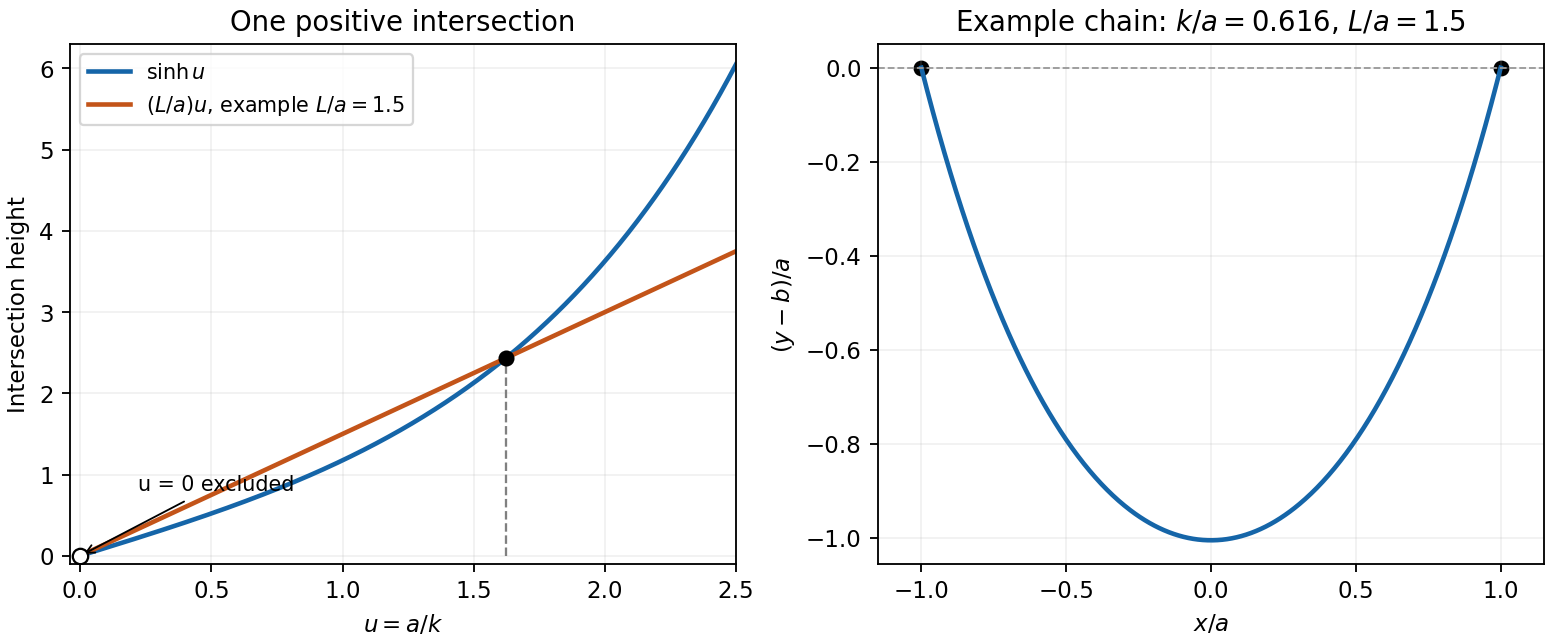
Unique positive catenary parameter from a hyperbolic-sine intersection, with an example hanging chain
. Details. 
More explicitly, has derivative , because the numerator vanishes at zero and has derivative . Since and , every yields exactly one positive , hence exactly one positive .
For an eigenfunction in the operator domain, . Substitution into the Rayleigh quotient givesThe cancellation only needs a finite nonzero norm; orthonormalization makes both denominator and norm equal to one.
Assume is self-adjoint on its specified operator domain, and the admissible variations preserve that domain and any boundary conditions, so no boundary terms spoil self-adjointness. Let . The first variation of the Rayleigh quotient isAt , the residual vanishes, so . More explicitly, for a normalized and ,For a fixed admissible direction scaled by a small parameter, the change is second order. This is stationarity, and is not necessarily a minimum for an excited state.
Conversely, vanishing first variation for every admissible complex direction yields the stationary equationAt the original stationary point, this is . The printed equation with an arbitrary perturbed in the final factor is not generally true. Taking with gives , even though the first-order change in is zero. Thus the valid claim is the stationary equation at the extremal state, not an exact eigenvalue equation for every variation.
Assume a complete orthonormal eigenbasis and a self-adjoint operator bounded below, with the trial state in its operator domain or associated energy-form domain. The expansion and orthogonality giveConsequentlyIt is a weighted average of eigenvalues, all at least . This is the Rayleigh-Ritz variational principle; equality holds precisely when the trial state lies in the ground-state subspace. A continuous part of the spectrum would require the corresponding spectral integral in place of part of the sum.
Use the intended infinite square well interpretation: the kinetic-energy operator on with zero Dirichlet boundary conditions. The variational energy is most safely evaluated through its quadratic form,The boundary term vanishes because the trial function vanishes at both walls. Its zero extension has derivative jumps there, so the form interpretation avoids assigning an unrestricted full-line second derivative to it.
Set and . Apart from an irrelevant factor , the trial function is . Polynomial integration givesHence the polynomial Rayleigh-Ritz trial space for a one-dimensional box has energyThe denominator is strictly positive, since . Differentiation givesThe two stationary parameters are . The smaller is a local maximum; the larger is a local minimum. Since the energy tends to as , the latter is the global minimum:The upper stationary value is . Exact roots give a slightly tighter bound than substituting the rounded hints.
There are two qualifications to the printed operator and comparison energy. For the box with Dirichlet boundary conditions and width , the actual ground-state energy iswhich lies just below the variational result. The coefficient printed as an exact eigenvalue is inconsistent with this box problem. Also, merely declaring the differential expression to be zero outside the interval does not impose hard-wall confinement or specify a self-adjoint domain. Read literally on a space admitting exterior-supported states, it has zero-energy states outside and does not have the claimed positive ground energy. The boxed variational result is the well-defined answer for the intended confined particle; a different full-line operator would need its domain and matching conditions supplied.
Articles by others on the same topic
There are currently no matching articles.