Past exam of the options II course of the University of Oxford / 2005 (AO2, XMAT 4304)

This University of Oxford Part A options paper covers fourteen printed sections and nineteen questions. ^[ref] The archive contains the complete editable eleven-page transcription. Bounded official-source searches found no advertised answers to this exact paper. All 30 source leaves and their unnumbered tasks are covered below. The source's mechanics potential is retained in the transcription, and its physical interpretation is qualified in the solution. The string-length and statistical-distribution assumptions are also made explicit where needed.

Count the pairs $(g,\omega )$ for which $g$ fixes $\omega$. Counting first by group elements gives ${\sum }_g\mathrm{Fix}(g)$, while counting first by points gives ${\sum }_{\omega }|\mathrm{Stab}(\omega )|$. On a group orbit of size $r$, orbit-stabilizer theorem makes each stabilizer have size $|G|/r$, so that group orbit contributes $|G|$ to the second sum. Dividing by $|G|$ proves Burnside's lemma:A tetrahedron has four vertices. A rotational symmetry is determined by the image of one vertex, with four possibilities, and the cyclic orientation of the three vertices around it, with three possibilities. All these choices are realizable, so its rotational symmetry group of a tetrahedron has order $12$. More explicitly, its elements are the identity, the two nontrivial rotational symmetries around each of four vertex-to-opposite-face axes, and the half-turn about each of three axes through opposite edge midpoints. Thus there is one element of order 1, eight of order 3, and three of order 2. The induced permutations of vertices are the even permutations, identifying the group with $A_4$.

Apply the group action to the set of edge colourings. A colouring is fixed by a rotational symmetry precisely when its colour is constant on each cycle of the induced edge permutation. The identity has six edge cycles and fixes $4^6$ colourings. A vertex-axis rotational symmetry has two cycles of length three, fixing $4^2$. An opposite-edge half-turn fixes the two edges on its axis as sets and exchanges the other four in two pairs, giving four cycles and $4^4$ fixed colourings. ThereforeReflections are excluded because the equivalence in the source uses rotational symmetries.

Map the integers into a field by $n\mapsto n1$. Its kernel is a prime ideal of $\mathbb{Z}$, since the image has no zero divisors. Thus the kernel is either zero or $(p)$ for a prime $p$. In the zero case, the map extends injectively to the rational numbers by taking quotients of nonzero integers. In the other case, its image is the field ${\mathbb{F}}_p$. This proves the prime-field assertion.

A finite field cannot contain the infinite rational field, so it has characteristic $p$. It is a finite-dimensional vector space over its prime field ${\mathbb{F}}_p$, say of dimension $n\ge 1$, and choosing a basis counts its elements asFor existence, put $q=p^n$ and take a splitting field of $x^q-x$ over ${\mathbb{F}}_p$. Its derivative is $-1$, so it has exactly $q$ distinct polynomial roots. The polynomial roots are closed under addition and multiplication because the Frobenius identity gives $(u+v{)}^q=u^q+v^q$ and $(uv{)}^q=u^q{v}^q$. They include $0,1$, are closed under additive inverses, and for a nonzero polynomial root $u$, $(u^{-1}{)}^q=(u^q{)}^{-1}=u^{-1}$. They therefore form a field of exactly $q$ elements. Indeed this field is the splitting field because it contains all polynomial roots and is generated by them.

In order 4, characteristic is 2. For $\omega \ne 0,1$, the multiplicative group has order 3, so ${\omega }^3=1$ and ${\omega }^2\ne 1,\omega$. Factorization of $x^3-1$ gives ${\omega }^2+\omega +1=0$. The quadratic $x^2+x+1$ has no polynomial root in ${\mathbb{F}}_2$ and is the minimal polynomial. Write $s={\omega }^2=\omega +1$. The complete tables areFor an element $\xi \ne 0,1$ in order 8, the tower law makes $[{\mathbb{F}}_2(\xi ):{\mathbb{F}}_2]$ divide3. It is not1, so its minimal polynomial is an irreducible monic cubic. Its constant term must be1. A cubic $x^3+a{x}^2+bx+1$ has no polynomial root at 1 exactly when $a+b=1$, and absence of a polynomial root is equivalent to cubic irreducibility. Consequently the two possibilities areBoth occur: together with $x$ and $x+1$ they factor $x^8-x$ over ${\mathbb{F}}_2$, whose distinct polynomial roots are exactly the eight elements of the field. Each cubic contributes its three polynomial roots.

Euler's totient function $\varphi (n)$ counts the integers $1\le a\le n$ coprime to $n$, equivalently the invertible residue classes modulo $n$. Among $1,\dots ,p^e$, exactly the $p^{e-1}$ multiples of $p$ are not coprime to the prime power. HenceFactor $n={\prod }_p{p}^{e_p}$. Its distinct prime-power factors are pairwise coprime, so the permitted multiplicativity givesFor $n=1$, the empty product is one and agrees with $\varphi (1)=1$.

Use prime factorization and multiplicativity to check the identity one prime at a time. Fix $p$ and put $a=v_p(m)$, $b=v_p(n)$, $r=\min (a,b)$. The local factors to compare areIf either exponent is zero, $r=0$ and the equality follows from $\varphi (1)=1$. If both are positive, the prime-power formula makes both sidesMultiplying the local identities over all primes and using $\gcd (m,n)={\prod }_p{p}^{\min (v_p(m),v_p(n))}$ givesThis accounts for repeated prime factors shared by the two inputs, which ordinary coprime multiplicativity alone would not remove.

Fermat's little theorem states that for a prime $p$ and an integer $a$ not divisible by $p$,Equivalently, $a^p\equiv a(\mathrm{mod}p)$ for every integer $a$, with divisibility by $p$ allowed in that latter formulation.

Since $n>1$, its factorial is even, so $(n!{)}^2+1$ is odd and its prime divisor $p$ is odd. Also $p$ cannot divide $n!$, since it would then divide1. Modulo $p$,Raise this equation to the integer power $(p-1)/2$. Fermat's little theorem givesAs $p$ is odd, $1$ and $-1$ are distinct residues. Thus the exponent is even, and

If a prime divisor $p$ of $(n!{)}^2+1$ satisfied $p\le n$, it would divide $n!$ and therefore divide the difference $(n!{)}^2+1-(n!{)}^2=1$, impossible. Hence $p>n$.

Every integer $(n!{)}^2+1>1$ has a prime divisor, and (ii) makes each of its prime divisors congruent to 1 modulo 4. Taking arbitrarily large $n$ produces such primes beyond every bound. ThereforeEquivalently, if their list were finite, choosing $n$ at least its largest member would produce a new member larger than that supposed maximum.

The monotone convergence theorem says that if $0\le f_n\uparrow f$ almost everywhere and the functions are measurable on a measure space, thenwith infinite integrals permitted. The limit is measurable after the usual modification on any exceptional null set.

The dominated convergence theorem says that if measurable functions $f_n$ converge almost everywhere to $f$ and satisfy $|f_n|\le g$ almost everywhere for an integrable nonnegative function $g$, then $f$ is integrable andThe theorem applies equally to real or complex functions. In particular domination must be by one fixed Lebesgue integrable function, rather than by a different bound for each $n$.

Put $G_N={\sum }_{n=1}^N|f_n|$. These are nonnegative measurable functions increasing to $G={\sum }_{n=1}^{\infty }|f_n|$, possibly initially with value infinity. Monotone convergence theorem givesAn infinite value on a set of positive measure would force an infinite integral. Thus $G$ is finite almost everywhere and, after setting it to zero on its null exceptional set if desired, is integrable.

Where $G$ is finite, the real series ${\sum }_n{f}_n$ is absolutely convergent. Define its sum to be $h$ there and zero on the exceptional null set. Measurability follows as an almost-everywhere limit of partial sums, and $|h|\le G$ almost everywhere gives integrability. Every partial sum is dominated by $G$, so dominated convergence theorem yieldsIn fact the convergence is also in the integrable-function norm:

Use $|\sin (\alpha x)|\le |\alpha |x$ for $x\ge 0$. For the source's functions,The last integral follows by the substitution $u=nx$ and integration by parts. Since ${\sum }_n{n}^{-2}$ converges, (ii) permits summing the integrals and identifies an integrable almost-everywhere sum.

For every $x>0$, the geometric series givesThe functions vanish on $x\le 0$, and the single endpoint does not change the integral. Use the supplied integral of $f_n$ to obtainThe estimates include negative $\alpha$ through its absolute value, and the case $\alpha =0$ gives zero on both sides.

Fubini's theorem for the product of two sigma-finite measure spaces states that an integrable measurable function on the product has integrable sections almost everywhere, the section integrals define Lebesgue integrable functions, and both iterated integrals equal the product integral. The integrability hypothesis is absolute integrability. For nonnegative measurable functions, Tonelli's theorem gives equality of the possibly infinite product and iterated integrals without first assuming finiteness.

The displayed function is not Lebesgue integrable. Its value at the origin can be assigned arbitrarily, since a point is a null set. On $0<x<1$ and $0<y<x/2$,Consequently Tonelli's theorem gives the divergent lower boundThe signed iterated integrals illustrate why the hypothesis matters. For $x>0$, $f(x,y)={\partial }_y[y/(x+y{)}^2]$, so integration first in $y$ and then in $x$ gives $1/2$. Integrating first in $x$ gives $-1/2$, using $f(x,y)=-{\partial }_x[x/(x+y{)}^2]$. Exceptional boundary sections have measure zero. Thus finite iterated values do not establish product integrability.

Choose measurable versions of the two Lebesgue integrable functions and consider $F(x,y)=g(x-y)h(y)$. Translation and the corresponding linear change of variables preserve Lebesgue measurability; one can first use Borel versions and then disregard the resulting null-set changes. Tonelli's theorem and translation invariance giveFubini theorem therefore shows that the section in $y$ is integrable for almost every $x$. Define $(g\ast h)(x)$ by that section integral where it exists and by zero on the exceptional null set. Fubini theorem also makes this a measurable Lebesgue integrable function, withIts almost-everywhere defining formula is precisely the desired convolution. This construction explains why an everywhere-existing pointwise integral is not required.

For fixed real $t$, multiplication by $e^{itx}$ does not change the absolute value. The product integrability proved in (ii) therefore justifies Fubini theorem in the following calculation. Set $u=x-y$ in the inner integral:ThusThe positive exponential convention in the source is used throughout; no normalization factor is introduced under that convention.

The product topology on $X\times Y$ has the open rectangles $U\times V$, with $U$ open in $X$ and $V$ open in $Y$, as a topological basis. The projection preimages are $p_X^{-1}(U)=U\times Y$ and $p_Y^{-1}(V)=X\times V$, so both projections are continuous.

If $f:Z\to X\times Y$ is continuous, both coordinate compositions are continuous. Conversely, if both are continuous, thenis open for every basic rectangle, proving continuity of $f$. Given paths between two chosen endpoints in each factor, their coordinatewise pair is therefore a continuous path in the product, proving that a product of path-connected spaces is path-connected.

For the compact-neighborhood assertion, fix $x\in K$. For each $y\in L$, choose an open rectangle $U_y\times V_y$ containing $(x,y)$ inside $W$. Compactness of $L$ chooses finitely many $V_{y_j}$ covering $L$. PutThen $x\in U_x$, $L\subseteq V_x$, and $U_x\times V_x\subseteq W$: any point of $V_x$ belongs to one of those rectangles' second factors, while $U_x$ lies in every first factor.

Compactness of $K$ now selects finitely many $U_{x_i}$ covering $K$. SetThese are open, contain $K$ and $L$, and if $(u,v)\in U\times V$, choose an $i$ with $u\in U_{x_i}$ and use $v\in V_{x_i}$. HenceIf $K$ or $L$ is empty, take the corresponding open factor empty and the other factor the whole space; the assertions then hold directly. No Hausdorff assumption on the factors is needed.

A Hausdorff space separates any two distinct points by disjoint open neighborhoods. For a subspace $A\subseteq X$, intersect such neighborhoods in $X$ with $A$ to obtain disjoint neighborhoods in the subspace topology. Thus subspaces inherit the Hausdorff property.

If $(z_1,z_2)$ lies off the diagonal of a Hausdorff space's square, choose disjoint open neighborhoods $U$ of $z_1$ and $V$ of $z_2$. The open rectangle $U\times V$ contains the pair and avoids the diagonal. Therefore its complement is open and the diagonal is closed.

The map $F:X\times Y\to Z\times Z$ given by $F(x,y)=(f(x),g(y))$ is continuous by the coordinate criterion from E3. The equality locus is $F^{-1}({\Delta }_Z)$ and is closed as an inverse image of a closed set.

Let $q:X\to X/\sim$ be the quotient map. If the quotient is Hausdorff, apply the same argument to $q$ in both coordinates:is closed in $X\times X$.

Conversely suppose $R$ is closed and $q$ is open. Take two distinct quotient points, with representatives $x,y$. Since $(x,y)\notin R$, an open rectangle $U\times V$ around it avoids $R$. The images $q(U)$ and $q(V)$ are open quotient neighborhoods. They are disjoint, because a quotient point in their intersection would have equivalent representatives $u\in U$, $v\in V$, giving $(u,v)\in R$. Hence the quotient is Hausdorff. Thus closedness of the relation and openness of the quotient map suffice for a Hausdorff quotient.

A sufficient regular-level condition is $\nabla f(x)\ne 0$ at every point with $f(x)=0$. The implicit function theorem then makes the zero level a two-dimensional continuously differentiable submanifold. Its tangent space isFor a minimizing pair $(a,b)$ and any tangent vector $v\in T_a{S}_f$, take a differentiable surface curve $x(s)$ with $x(0)=a$, $x^{\prime }(0)=v$. The function $\Vert x(s)-b{\Vert }^2$ has a minimum at zero, so its derivative $2(a-b)\cdot v$ vanishes. Varying the other point similarly proves orthogonality to $T_b{S}_g$.

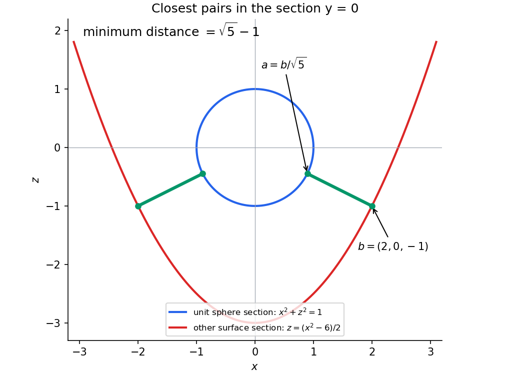
For the particular surfaces, minimize the distance from the origin to the second surface first. Put $u=x^2$, $v=y^2$, so $u,v\ge 0$ and $z=(u-v-6)/2$. ThenLet $s=u-v$. Since $u+v\ge |s|$, this is at least $|s|+(s-6{)}^2/4$, with equality when one of $u,v$ is zero. For $s\ge 0$, this quadratic has its minimum at $s=4$, with value 5. For $s\le 0$, it decreases up to zero and has minimum9 on that half-line. The global minimum is therefore5, attained atAll points of this surface lie outside the unit sphere. For any such $b$, the distance to the sphere is $\Vert b\Vert -1$, attained at $a=b/\Vert b\Vert$ by the triangle inequality. ConsequentlyThis is a global minimization, not merely a stationary-point calculation.

Write $I[y]={\int }_a^{b}G(x,y,y^{\prime })dx$. For endpoint-zero variations $\eta$, the first variations areFor a normal constrained extremal, choose a variation ${\eta }_0$ with $\delta I({\eta }_0)\ne 0$. Given any $\eta$, use the implicit function theorem to choose a small correction in the ${\eta }_0$ direction so that $y+t\eta +s(t){\eta }_0$ preserves the constraint. Differentiating it and the stationarity condition at zero givesIntegrate the derivative-of-variation term by parts. Since the variations vanish at both endpoints, the boundary term is zero. The fundamental lemma of the calculus of variations then givesThe regularity condition on the constraint is what permits the coefficient of $F$ to be normalized to 1. In a degenerate case, the general multiplier statement uses ${\lambda }_{0}F-{\lambda }_{1}G$ with the two coefficients not both zero; the source's displayed form is the normal case.

For a string described as a function graph $r(x)=(x,y(x))$, its arc-length element is $|r^{\prime }(x)|dx=\sqrt{1+y^{\prime }(x{)}^2}dx$. Inextensibility therefore givesThis also forces $l\ge 2a$, with equality only for the straight function graph.

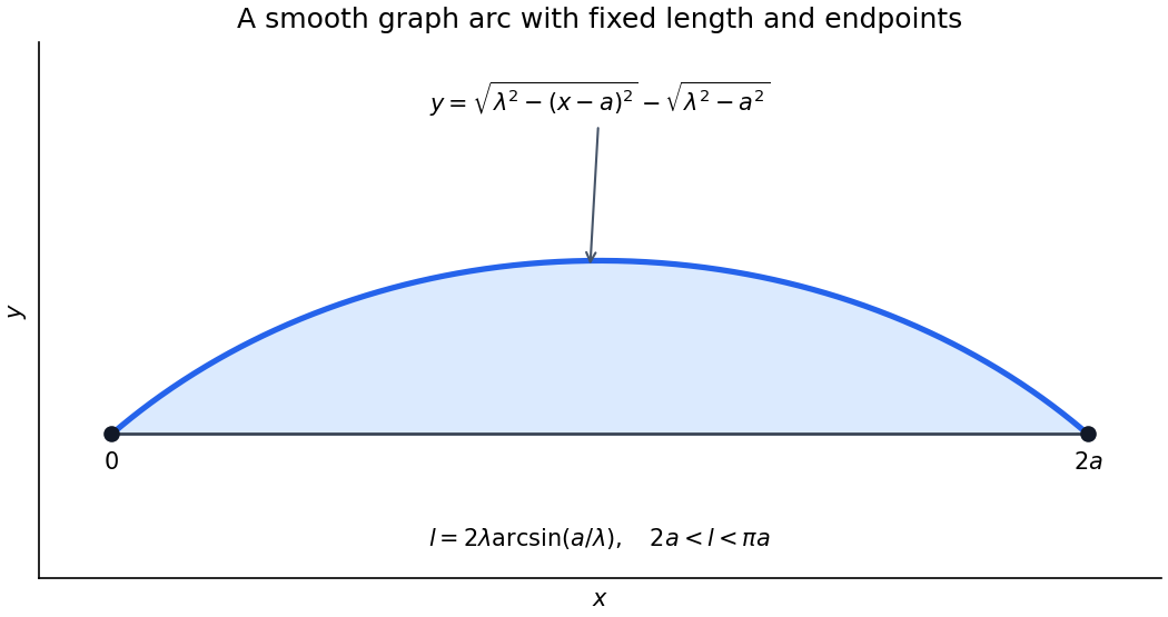
For the upper function graph, the vertical cross-section of the enclosed region has length $y(x)$, so its area is $J[y]={\int }_0^{2a}y(x)dx$. A maximizing nonnegative arch therefore uses $F=y$ and $G=\sqrt{1+y^{\prime 2}}$ in the normal Euler-Lagrange equation. It becomesIntegrating once gives $y^{\prime }/\sqrt{1+y^{\prime 2}}=(c-x)/\lambda$. The concave upper branch has $\lambda >0$ and integrates to $y=\sqrt{{\lambda }^2-(x-c{)}^2}+d$. The equal zero endpoint heights force $c=a$ and $d=-\sqrt{{\lambda }^2-a^2}$. HenceIt is a circular arc. To find its parameter, substitute into the length integral: $\sqrt{1+y^{\prime 2}}=\lambda /\sqrt{{\lambda }^2-(x-a{)}^2}$, givingThis scalar equation determines $\lambda$ numerically when needed; no explicit solution is required.

The arch is a global maximum in its smooth function graph regime. For $\lambda >0$, the integrand $y-\lambda \sqrt{1+y^{\prime 2}}$ is concave and strictly concave in its slope. Its supporting-tangent inequality, integrated against any competing function graph with the same endpoint values, has first-order term zero by the Euler-Lagrange equation. Thus $J[y]-\lambda I[y]\le J[y_{\ast }]-\lambda I[y_{\ast }]$. On the fixed-length class this is $J[y]\le J[y_{\ast }]$; strict slope concavity also gives uniqueness.

The source leaves the length range implicit. A twice continuously differentiable function graph of this form needs $\lambda >a$, giving $2a<l<\pi a$. At $l=2a$ the straight function graph is the degenerate solution. The semicircle limit $l=\pi a$ has vertical endpoint tangents and is outside that smooth function graph class. For $l>\pi a$, no arc in the claimed smooth function graph family exists, so the stated formula cannot describe a twice continuously differentiable maximizing function graph under those unrestricted data. Allowing overhanging curves changes the admissible class.

Write the position of a mass element relative to the centre of mass as $r$. Expand its squared velocity and integrate:The mixed term vanishes because $\int rdm=0$. Alsousing the scalar triple-product identity. ThereforeIn principal axes the inertia tensor is diagonal, so the second term is $\frac{1}{2}(A{\omega }_1^2+B{\omega }_2^2+C{\omega }_3^2)$. Substituting the three Euler-angle components given in the source gives its displayed kinetic-energy expression directly.

For $A=B$, the first two component squares have opposite mixed terms and sum to ${\dot{\theta }}^2+{\dot{\varphi }}^2{\sin }^2\theta$. Put $n=\dot{\psi }+\dot{\varphi }\cos \theta$. Using the orientation-dependent potential printed in the source therefore gives the formal modelThe cyclic coordinates $x,y,\psi$ have conserved momenta $M\dot{x},M\dot{y},Cn$. Consequently $\dot{x},\dot{y},n$ are constant. The coordinate $\varphi$ is also cyclic, withFor imposed fixed tilt $\theta =\alpha \in (0,\pi /2)$, conservation of $n$ and $p_{\varphi }$ forces $\dot{\varphi }=\Omega$ constant. Impose the fixed-height condition $z=h$ in this formal constrained model. Its $\theta$ equation isSet the tilt constant and divide by its nonzero sine. This givesA real polynomial root requires its quadratic discriminant to be nonnegative:When this condition holds the two algebraic rates are $(Cn\pm \sqrt{C^2{n}^2-4AMgh\cos \alpha })/(2A\cos \alpha )$.

There is a physical inconsistency in the printed data that must be kept distinct from this algebra. If $(x,y,z)$ are literally Cartesian coordinates of the centre of mass in uniform gravity, the gravitational potential is $Mgz$, not $Mgz\cos \theta$. The printed Lagrangian consequently does not follow from that Cartesian-height interpretation. Moreover its unconstrained $z$ equation is $\ddot{z}=-g\cos \theta$, so constant height at the indicated tilt requires a constraint reaction. The requested rate and discriminant follow from the printed orientation-dependent potential with fixed height imposed; a standard heavy-top interpretation instead uses a height proportional to an axis distance times $\cos \theta$, with the reference point and corresponding inertia specified consistently. The kinetic-energy derivation is independent of this source inconsistency.

Set $u=r\psi$, choose $\alpha >0$ for a negative bound-state energy, and write $\kappa =2mK/{\hslash }^2$. Multiplying the radial equation by $r$ givesFor $u=e^{-\alpha r}f$, its second derivative is $e^{-\alpha r}(f^{\prime \prime }-2\alpha f^{\prime }+{\alpha }^{2}f)$. Substitution cancels the two ${\alpha }^2$ terms and givesFor the physical hydrogen problem, the angular eigenvalue has $\ell$ a nonnegative integer. Regularity at the origin selects the Frobenius exponent $u\sim r^{\ell +1}$, rather than the singular branch. PutThe equation for the series factor $v=f/r^{\ell +1}$ is $r{v}^{\prime \prime }+(2\ell +2-2\alpha r)v^{\prime }+(\kappa -2\alpha (\ell +1))v=0$, and coefficient comparison yieldsThe regular confluent-hypergeometric solution generically grows like $e^{2\alpha r}$ in this series factor; after the extracted $e^{-\alpha r}$ it is not normalizable. A bound state requires termination at some degree $q\ge 0$, namely $2\alpha (q+\ell +1)=\kappa$. Thus $n=q+\ell +1$ is an integer greater than $\ell$, andRegularity, normalizability and the integer angular index are the physical conditions selecting this spectrum; the differential equation without those conditions would admit many other solutions.

For $n=1$, necessarily $\ell =0$ and $q=0$. With $a_0={\hslash }^2/(mK)$,A normalized spatial ground state is ${\Psi }_1=(\pi a_0^3{)}^{-1/2}{e}^{-r/a_0}$. In spherical coordinates the radial probability has weight $r^{2}dr$. Constants and the angular integral cancel in the tail ratio. The supplied integral with $\lambda =2/a_0$ gives

Milne-Thomson's circle theorem inserts an impermeable circular boundary into a two-dimensional irrotational incompressible flow. If $f(z)$ is analytic in a neighborhood of the closed disc and its flow singularities lie outside, the new complex potential outside $|z|=a$ isReflection and coefficient conjugation make the second term analytic outside the circle, with its image singularities inside. On $|z|=a$, $a^2/\bar{z}=z$, so the two terms sum to $2\mathrm{Re}f(z)$: the streamfunction is constant there. Thus no velocity crosses the circle. At infinity the image term tends to the constant $\overline{f(0)}$, which has no effect on velocity, and the far-field flow is retained. This proves the construction, with an additive potential constant immaterial.

Put $A=\mu e^{i\alpha }$, $B=\mu e^{-i\alpha }$. For the dipole the reflected potential is $B/(a^2/z-b)=Bz/(a^2-bz)$, givingIts image pole is $c=a^2/b$, inside the cylinder. The complex velocity isNear $c$, the second term is $C(z-c{)}^{-2}$ with $C=B{a}^2/b^2$, while $v_0(z)=-A/(z-b{)}^2$ is analytic there. The square of the pole term has no residue, nor does $v_0^2$. The cross term has residue $2C{v}_0^{\prime }(c)$, soTake the contour counterclockwise around the cylinder, as in the supplied Blasius force theorem. The residue theorem gives $\frac{1}{2}i\rho \oint (w^{\prime }{)}^{2}dz=-\pi \rho \mathrm{Res}(w^{\prime }{)}^2$. ThereforeThe force points toward the dipole. Its independence of dipole orientation follows from the product $AB={\mu }^2$ in the sole residue contribution.

Irrotational motion in this simply connected fluid region has a velocity potential, $u=\nabla \varphi$. Incompressibility gives $\nabla \cdot u=0$, hence $\Delta \varphi =0$.

The moving surface is a material surface: differentiating $y-\eta (x,t)=0$ along a particle gives ${\eta }_t+{\varphi }_x{\eta }_x={\varphi }_y$ at $y=\eta$. Linearizing about a flat stationary surface drops the product term and evaluates at zero, giving ${\eta }_t={\varphi }_y$ there. The Unsteady Bernoulli equation, after dropping quadratic velocity terms and absorbing the time-only constant into $\varphi$, is ${\varphi }_t+p/\rho +gy=0$. The linear capillary pressure at the surface is $p=-T{\eta }_{xx}$ relative to atmosphere, in the sign convention of the source. ThereforeFor $\eta =A\cos (kx-\omega t)$ choose the harmonic potential decaying at infinite depth,Its vertical derivative at zero equals $A\omega \sin (kx-\omega t)={\eta }_t$. Substitution into the dynamic condition gives $-{\omega }^2/k+g+T{k}^2/\rho =0$. ThusThe two positive terms are the gravitational and capillary contributions to the restoring force.