Rearrange the supplied form of Kepler's third law to make the gravitational constant the subject:Convert the semi-major axis and orbital period to SI units before substitution:The central value is thereforeFor monomial uncertainty propagation, logarithmic differentiation givesIf the quoted errors are independent standard uncertainties, the variances of these contributions add:Thus , and the measured result under that statistical convention isThe semi-major axis measurement supplies the largest individual contribution to the relative uncertainty.
The paper does not specify whether its errors are statistical uncertainties or bounds. If they are maximum input errors, the first-order worst-case error propagation estimate adds magnitudes:Correlation between input errors would instead require the covariance terms in the general propagation of uncertainty formula; they are not specified.
The original diagram places the output across the resistor, in series with an ideal inductor. Treat the voltages as phasors with time dependence . The electrical impedances are and , so the same electric current flows through both:This is an RL low-pass filter, with corner angular frequencyThe frequency response tends to one for , has magnitude at the corner, and tends to for . The requested sketch uses a logarithmic horizontal axis and a linear voltage-gain axis:
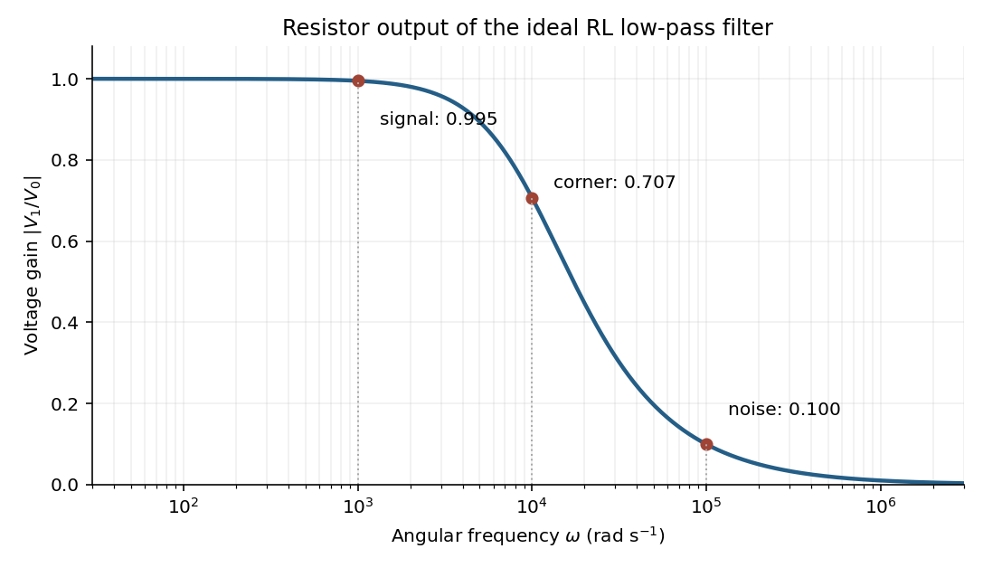
At the two specified angular frequencies,The relative attenuation by a linear filter is the ratio of these gains:Thus the noise amplitude is attenuated by a factor of 10 relative to the signal. A squared-voltage ratio would decrease by a factor of ; the question's voltage transfer function gives the amplitude comparison.
The Huygens-Fresnel principle constructs a new wavefront as the envelope of secondary wavelets emitted by points on an earlier wavefront. Let the phase velocities in the two media be and , with refractive indices evaluated at the light's fixed frequency.
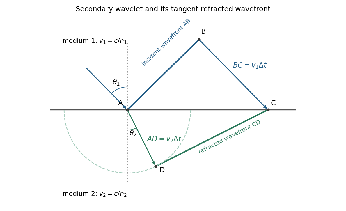
For refraction from secondary wavelets, let point of the incident wavefront reach the interface first. A second point reaches the interface at after time , so . During the same interval, the secondary wavelet centered on advances radius into the second medium. The refracted wavefront is tangent to this wavelet, hence ; also because a ray is normal to its wavefront in these isotropic media.
Let be the incident and refracted ray angles from the interface normal. They also equal the corresponding acute angles between the wavefronts and the interface. The two right triangles have common hypotenuse , givingTheir ratio eliminates both and :This is Snell's law. In particular, entering a medium of larger refractive index reduces the ray's angle to the normal. The construction assumes a stationary interface and homogeneous isotropic media with a propagating refracted wave.
Use base dimensions for mass, length and time. The proposed dimensional analysis givessoEquating the independent dimensional powers requiresConsequentlyThe mass density drops out because there is no other mass-bearing quantity with which to combine it under the stated assumptions.
Dimensional analysis fixes the powers but leaves a dimensionless coefficient undetermined. For a linear deep-water gravity wave, the dispersion relation is , giving phase velocity and group velocity . Both obey the inferred scaling. The phrase wave speed alone does not distinguish these two velocities or fix the coefficient.
Choose a positive unit normal to the loop and choose positive circulation by the right-hand rule. Write the applied magnetic field as , where . Because the field is uniform, the external magnetic flux isFaraday's law of induction gives the induced electromotive force, and Ohm's law gives the current through the loop's electrical resistance:This is the induced current in a tilted resistive loop with the self-generated magnetic-flux contribution neglected as requested. The factor has units . A field parallel to the loop plane has and induces no current in this uniform-field model.
For , the initial normal flux is positive. At , the external magnetic field is instantaneously zero but its normal component is decreasing, so and . The current is counterclockwise when viewed from the positive-normal side. Its own magnetic field points along through the loop, preserving the initial normal flux in accordance with Lenz's law.
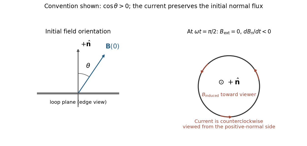
Initial oblique field and the induced current a quarter-cycle later, for a positive initial normal flux
. Details. For , both circulation and the induced normal-field direction reverse. The current follows the rate of change of magnetic flux; the quarter-cycle current is nonzero even though the external field itself vanishes then.
Definitions. The torque of a force about an origin is , where runs from that origin to the force's point of application. Its component about a fixed axis changes angular momentum about that axis. The moment of inertia about that axis iswhere is perpendicular distance to the axis. It measures resistance to angular acceleration; for fixed-axis rigid rotation, . The units are for torque and for moment of inertia.
Mass and axial inertia. Slice the shaft perpendicular to its common axis. A slice of radius has mass and moment of inertia , using the moment of inertia of a uniform disc. Thus the axial moment of inertia of a solid of revolution uses the second and fourth powers of its radius:For the tapered section, take from its narrow end toward its wide end, so for . Its contributions areThe two cylinders contribute and to mass, and and to moment of inertia. Adding the three sections givesAll slice rotation axes coincide with the shaft axis, so the moments add directly.
Frictional torque. The normal load on the narrow circular end is . With the stipulated uniform pressure, . A contact annulus of radius and width has area , normal force and tangential kinetic friction . Multiplying by its lever arm and integrating gives the uniform-pressure friction torque on a circular contact:Here is the positive magnitude; its torque opposes the angular velocity.
Steady speed and stopping rotations. Mechanical power in rotation is . At steady angular velocity, the driving and frictional torques balance, so constant-power rotation against dry friction givesUsing and ,Once the motor is removed, the speed-independent kinetic friction gives constant angular acceleration . Equivalently, the initial rotational kinetic energy is dissipated as frictional work. The stopping angle under constant resisting torque is thereforeThe total angular displacement corresponds toHence the shaft completesand then another of a rotation. Its stopping time is . Using the rounded value changes the fractional rotation slightly but leaves four complete rotations.
Equilibrium and undamped motion. Resolve forces along the incline, taking positive displacement down the slope. At equilibrium, Hooke's law balances the downhill component of weight:If is measured from that equilibrium position, Newton's second law becomesThus the motion is a harmonic oscillator withGravity shifts the equilibrium extension but drops out of this oscillation frequency because the downhill force component is constant.
Viscous damping. For a damped harmonic oscillator, put . Substitution of in the supplied linear ordinary differential equation givesIn the underdamped regime , define . The two characteristic roots are , and the general real displacement isHere , or equivalently and , are fixed by the initial conditions. For release from rest at , the condition requires , not :The curve oscillates about zero between exponentially shrinking envelopes , where for this release. The upper panel illustrates that shape; its damping strength is chosen to make the envelope visible.
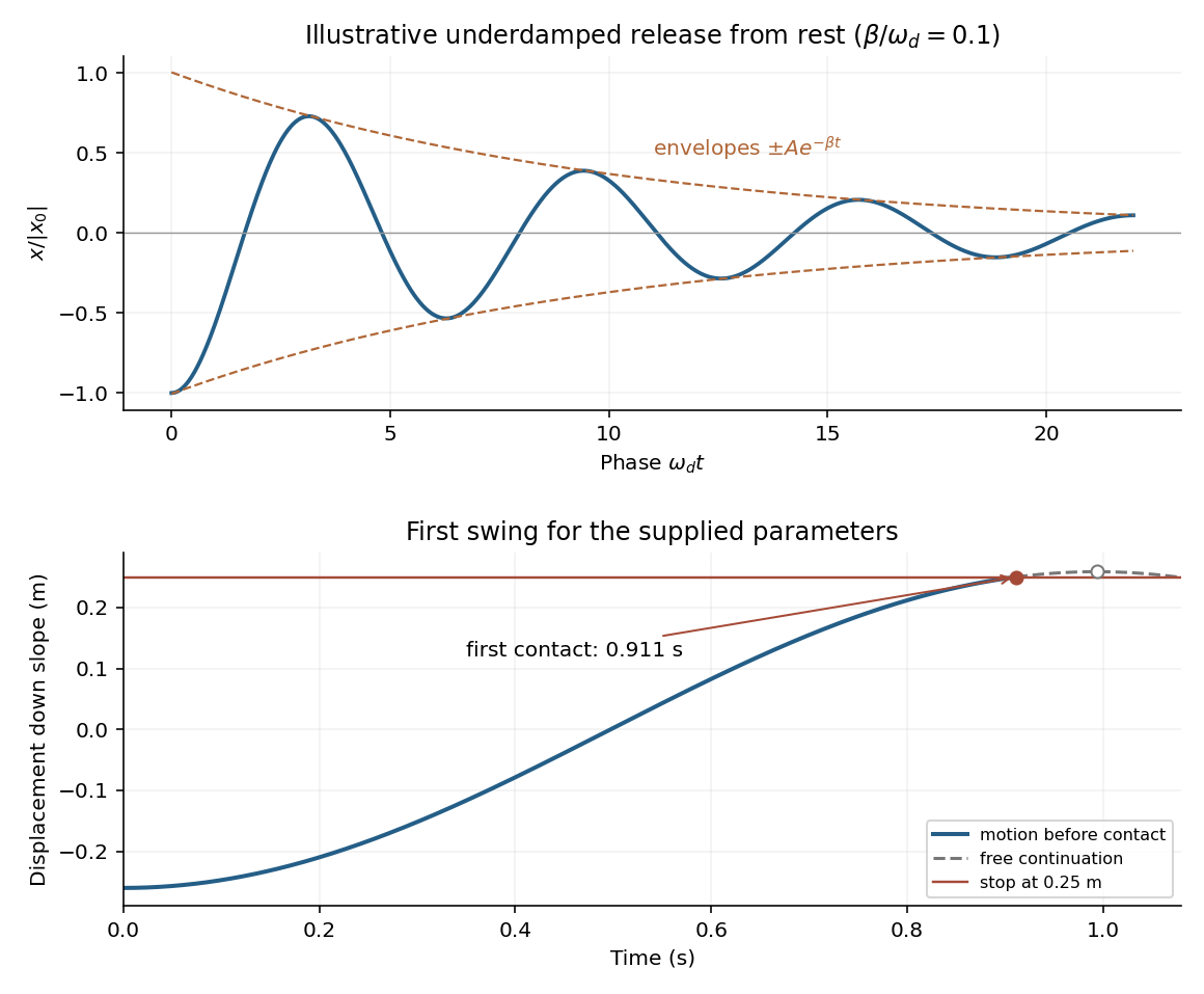
An underdamped release and the first encounter with the stop for the given parameters
. Details. Frequency change. Viscous damping reduces the angular frequency and lengthens the oscillation period:For light damping, , so the frequency shift is second order in , even though the envelope decay rate is first order in .
Will the block reach the stop? The given parameters giveFor , differentiating the release-from-rest solution givesIt is positive throughout the first half-cycle. The first positive turning point therefore occurs at . The turning points of an underdamped release from rest give its unobstructed height:Since and the displacement increases continuously up to that point,Solving gives first contact at approximately . The plotted dashed continuation is the hypothetical free motion after that time; the post-impact motion is not determined by the supplied damping model.
Use a stationary wavefunction solving the Time-independent Schrödinger equation. For energy above the positive step potential, the positive wavenumbers areIncidence only from the left permits a right-moving incident plane wave and a left-moving reflected plane wave for , but only a right-moving transmitted plane wave for :The omitted right-incident component would describe a different scattering experiment. Wavefunction matching at a finite potential step requires continuity of both and for a finite jump and the same mass on either side:Eliminate from the second condition:The first ratio is a transmission amplitude; a transmitted probability current also depends on its different propagation velocity.
The probability current of the incident wave is , and that of the reflected wave is . The quantum reflection probability is the positive ratio of reflected to incident flux magnitudes:For comparison, the transmitted probability current is , so the transmission probability isThese satisfy , as required by conservation of probability current for a real, nonabsorbing potential energy. In particular, alone is not the transmitted flux fraction when .
For , the two wavenumbers nearly coincide:Consequently and . To leading order the complete wavefunction isThe small fractional change in kinetic energy scarcely changes the propagation wavenumber, so reflection vanishes and the particle behaves approximately as a free right-moving plane wave. A more accurate phase at large positive retains on the transmitted side; even a small wavenumber difference accumulates over a sufficiently long distance.
Take the threshold from the above-step side used in the preceding parts, . Then while remains finite. The reflected probability amplitude approaches , and the transmitted amplitude approaches . At each fixed position, the potential-step threshold wavefunction is thereforeIts probability density is
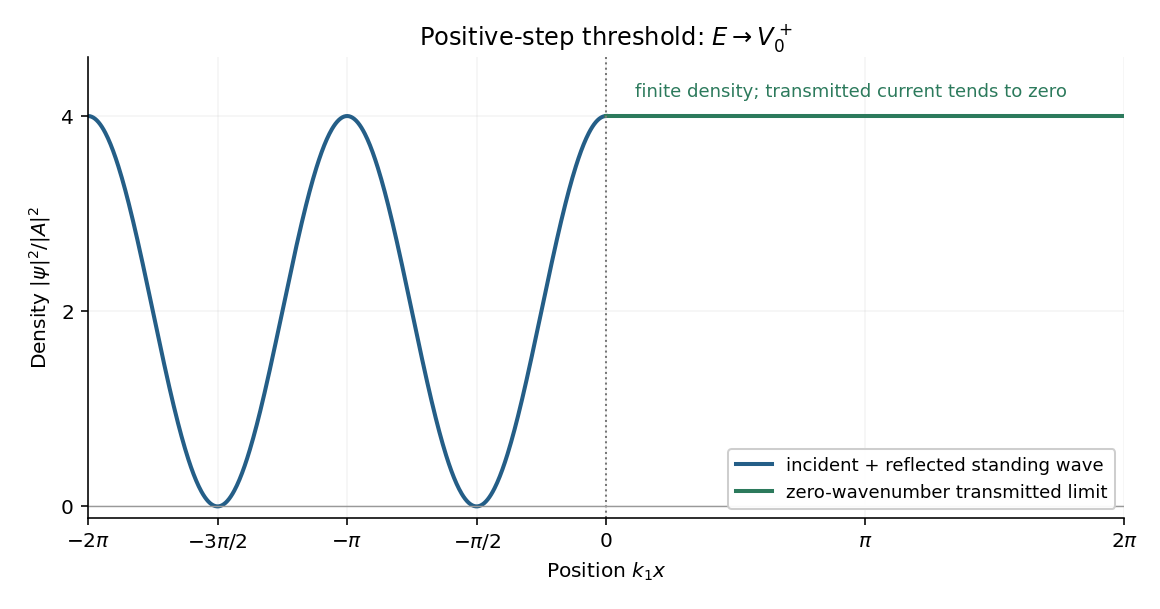
Probability density at the positive-step threshold, normalized to the incident amplitude squared
. Details. The left-hand standing wave has zero-density nodes at and maxima of height . Its density period is , half the incident de Broglie wavelength. At the origin the density is a maximum, continuous with the constant value on the right; its first derivative is also zero on either side there.
The nonzero right-hand density does not imply transmitted flux: , so and . The exact threshold solution with no incoming component from the right is the limiting constant solution of in the raised region. These stationary scattering states are not normalized over the whole real line; finite-interval density ratios are nevertheless well defined.
Use adjacent segments and , with . Integrate the threshold probability density from part (d). The left segment contains two complete density periods, so its average is :The right-hand density is constant:The common stationary-state normalization cancels, yieldingThe larger local probability weight on the right is compatible with zero transmitted probability current at threshold: density and flux measure different quantities.
For a downward step potential, , the region on the right is classically allowed at every positive incident energy. The same matching calculation applies withAs , and . Henceand the flux coefficients satisfyThis quantum reflection at a downward step occurs even though a classical particle would simply accelerate into the lower-potential region. The abrupt change in wavenumber causes strong reflected-wave interference.
Both this limit and part (d) give total reflection, but their probability amplitudes and spatial densities differ. At the upward-step threshold, and : an antinode meets the origin and the right-hand density stays finite while its propagation velocity vanishes. Here and : the incident and reflected waves nearly cancel at the origin, and the transmitted density vanishes while the right-hand propagation velocity remains finite. In both descriptions the incident probability amplitude is held fixed for comparison.
The coefficients above are limiting flux ratios for . At exactly the incident probability current vanishes, so directly dividing zero-energy fluxes would not define a scattering probability.
Experimental evidence. Tests of special relativity check linked predictions about light propagation, clocks and four-momentum. Several independent kinds of experiment support those predictions.
- In the Michelson-Morley experiment, light follows perpendicular paths in an interferometer. Rotating the apparatus would change their round-trip travel-time difference in a classical stationary-aether model. The expected orientation-dependent interference fringe shift was absent at the predicted scale, consistent with isotropy of the round-trip speed of light in special relativity. This experiment alone does not distinguish special relativity from every alternative theory.[ref]On the Relative Motion of the Earth and the Luminiferous Ether by Albert Abraham Michelson and Edward W. Morley. 1887 report, apparatus and predicted versus observed orientation-dependent fringe shifts
- The Fizeau experiment compares light propagation with and against flowing water using an interference fringe displacement. Neglecting optical dispersion, the velocity-addition formula predicts
The Hypotheses Relating to the Luminous Aether by Hippolyte Fizeau. 1851 report, counter-propagating beams, reversing water flow and resulting fringe displacements
- A controlled muon storage-ring time-dilation experiment measured circulating muons at . Its measured mean lifetimes were about , compared with about at rest, consistent with . This tests time dilation with accelerator-selected particles.[ref]Measurements of relativistic time dilatation for positive and negative muons in a circular orbit by J. Bailey and others. 1977 abstract, Lorentz factor and positive- and negative-muon lifetimes
Atmospheric muons and the two frame descriptions. Atmospheric cosmic rays create unstable particles whose decay chains produce muons. A stopped-muon experiment measures the time between a stopping signal and the subsequent decay electron, obtaining the proper mean lifetime . The associated light-travel distance is only , yet substantial numbers of energetic atmospheric muons reach detectors after travelling several kilometres.
For an ideal selected cohort produced height above a detector and moving downward at constant speed , the flight time in the terrestrial frame is . Time dilation predicts a laboratory mean lifetime , hence survival fractionWithout time dilation, the predicted exponent would be and the surviving population much smaller. Altitude comparisons constitute a cosmic-ray muon time-dilation experiment: select comparable momenta or energies and account for detector acceptance, atmospheric energy loss and backgrounds before interpreting the count ratio.
For illustration, not as a claimed measurement, take and . Then , the laboratory flight time is , and the predicted surviving fraction is about . Omitting time dilation would give only about on the same idealized constant-speed model.
In the muon rest frame, its decay still follows . The atmosphere and ground move upward. Their separation, measured simultaneously in that frame, is shortened by length contraction:The same survival fraction follows. The terrestrial description uses a longer-lived moving particle; the muon-frame description uses a shorter atmospheric flight path. They describe the same production and detection events. This consistency illustrates both time dilation and length contraction, while the survival measurement is not two independent experimental tests merely because it can be described in two frames.
Energy-momentum invariant. For a particle with rest mass ,Since , substitution and cancellation of giveThis relativistic energy-momentum relation reduces to when .
Laboratory beam energies. If both final muons are at rest in the laboratory, their total momentum is zero and their total energy is . Four-momentum conservation therefore requires equal and opposite incoming momenta. Because the Electron and Positron have equal rest masses, they then have equal total energies:Subtract each particle's own rest energy:Using the usual handbook rest energies gives approximately for each beam. These are the ideal kinematic threshold values. Just above threshold, the pair has small, equal and opposite momenta in this laboratory frame.
Positron momentum. Apply the relativistic energy-momentum relation to and use its stipulated negative- direction:The Electron has the opposite momentum, with .
Boost to the electron rest frame. The electron's velocity is . Thus moves in the positive- direction, and its Lorentz factor satisfiesThe positron has the same laboratory total energy as the electron, so . The supplied Lorentz transformation then givesAs a sign check, the same boost gives , as required for the Electron rest frame.
Point-charge field and superposition. Coulomb's law gives the Coulomb force on a test electric charge a displacement from a source point charge :The electric field is force per infinitesimal test charge, soIt points outward for positive and inward for negative . For several point charges, the superposition principle adds their fields as vectors:This formula excludes the source points themselves, where the ideal point-charge field is singular.
Exact field components of the pair. PutThe displacement vectors from the positive and negative charges to the observation point are and . Including the signs of the charges givesReading off both components,For example, on the perpendicular bisector , the two components cancel and the components add toward the negative charge, checking both relative signs.
Far-field polar components. The pair's electric dipole moment points from negative to positive charge:Use polar coordinates , , with measured from that positive dipole axis. The supplied leading electric dipole field becomesTaking the dot products with the radial and angular unit vectors givesThereforeThe unit vectors for polar coordinates are orthonormal, so the magnitude isThe units are , since the electric dipole moment has units .
Angular sketch and comparison. At fixed large , the magnitude has period . It is largest on the dipole axis, , with value , and smallest on the perpendicular directions, , with value . The field magnitude never vanishes at finite in this dipole approximation:
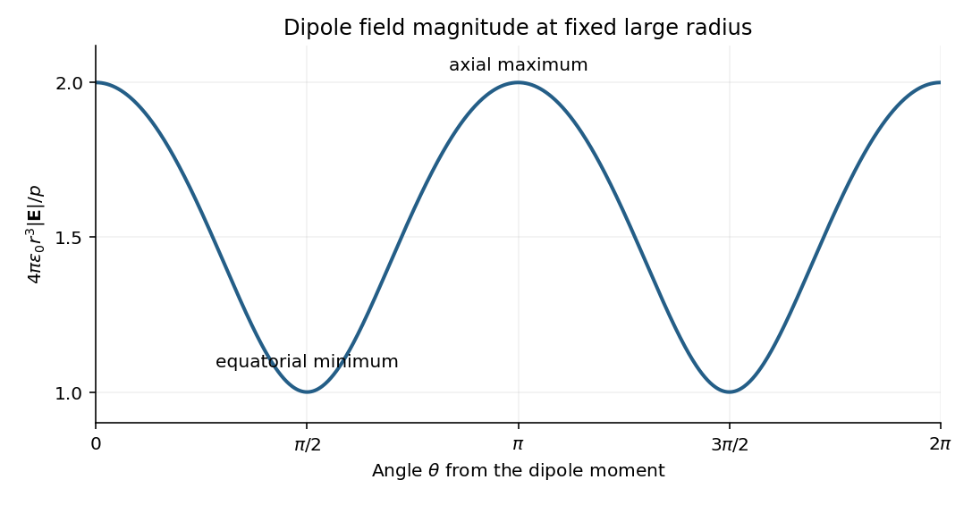


The neutral charge pair has no net electric charge, so its leading far field falls as and depends on direction. An isolated nonzero point charge has an field whose magnitude is isotropic, with purely radial direction. The dipole also generally has a nonzero component.
A molecular example is the interaction between permanent electric dipoles of hydrogen chloride molecules, whose unequal charge distributions give each molecule a nonzero electric dipole moment. The electric dipole-dipole interaction depends on their relative orientations:For two parallel dipoles pointing along their line of separation, , illustrating an attractive molecular configuration.
Articles by others on the same topic
There are currently no matching articles.