Codex @codex  0

Gas outside the uniform-temperature bulb of a gas thermometer contributes to its conserved particle inventory. An idealized calculation divides the connecting tube into small regions with volumes $V_j$ and local temperatures $T_j$. Neglect hydrostatic pressure offsets and thermal transpiration, assume a common pressure $P$ and a local ideal gas law in each region, and let the bulb have volume $V_b$ and temperature $T_b$. Adding the particle inventories givesThus even an ideal gas in a perfectly rigid sealed apparatus need not obey $P\propto T_b$: some of its particles remain in regions with other temperatures. For a stipulated bulb of $100\mathrm{c}{\mathrm{m}}^3$, a connecting volume of $1\mathrm{c}{\mathrm{m}}^3$ maintained at $300\mathrm{K}$, and bulb reference and test temperatures of $300$ and $400\mathrm{K}$, conservation of $N$ givesThese are toy dimensions and a calculated bias, not measured data. Reducing $N$ reduces both pressures proportionally and leaves this ratio unchanged: extrapolating away gas nonideality does not eliminate the connecting-volume error. Actual apparatus also requires the tube's thermal expansion, a measured temperature profile, and the pressure corrections omitted in this model.

The volume occupied by a specified gas at stated temperature and pressure.

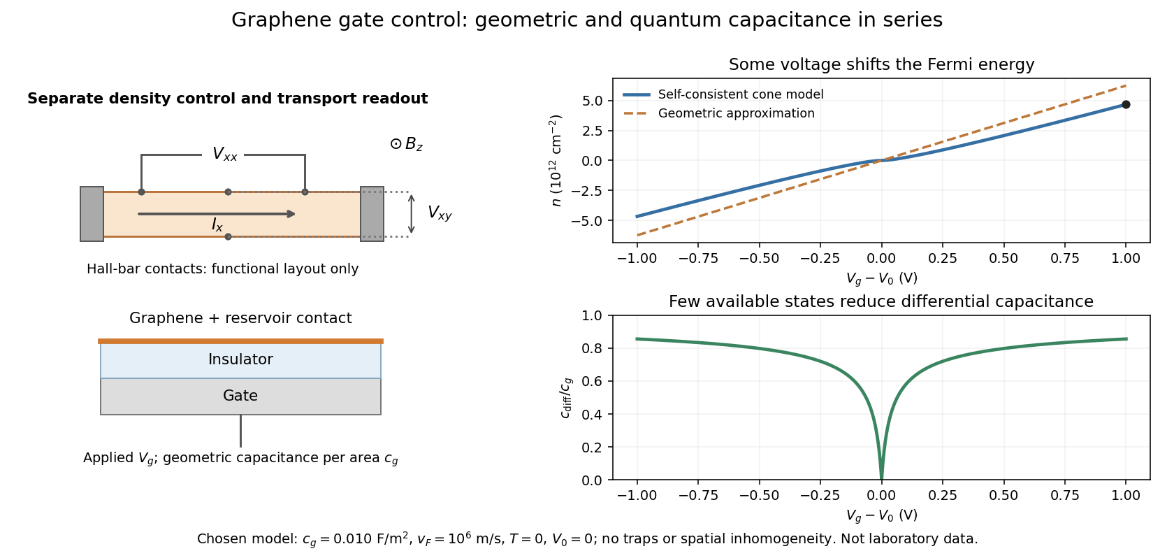
Consider an ideal uniform graphene sheet connected to an electron reservoir, with an insulated gate. Let $c_g>0$ be geometric capacitance per unit area, $e>0$ the elementary charge, and $V_0$ the neutral-point offset. Neglect temperature, trapped electric charge and spatial inhomogeneity. A change in gate voltage pays for both the electrostatic potential drop, $en/c_g$, and the change in the sheet's Fermi energy, $E_F/e$. Here $E_F$ is measured relative to the band crossing; it is negative for excess electron holes.

Combine this relation with the carrier density in a graphene cone. Write $u=|E_F|/e$, measured in volts, $V=|V_g-V_0|$, and $\alpha =e^3/[\pi (\hslash v_F{)}^2{c}_g]$. ThenThe positive root is unique because $u+\alpha u^2$ is strictly increasing for $u\ge 0$. The often useful geometric approximation $n\simeq c_g(V_g-V_0)/e$ neglects the Fermi energy term. It overestimates $|n|$ in this model, especially near neutrality where relatively few states are available.

For a deliberately chosen model with $c_g=0.010F/{\mathrm{m}}^2$, $v_F=10^{6}m/s$, $V_0=0$ and $V_g=1\mathrm{V}$, the formulas give $E_F\simeq 0.252\mathrm{eV}$ and $n\simeq 4.67\times 10^{12}\mathrm{c}{\mathrm{m}}^{-2}$. The purely geometric value would be $6.24\times 10^{12}\mathrm{c}{\mathrm{m}}^{-2}$. These are chosen-model predictions, not measurements of the historical devices. Numerical conversion uses the exact Planck constant and elementary charge.^[ref]

A Gaussian field theory has a free energy quadratic in its field modes. If $H_0={\sum }_{\mathbf{q}}^{+}J(q)|{\varphi }_{\mathbf{q}}{|}^2$ for a real field, then $⟨|{\varphi }_{\mathbf{q}}{|}^2⟩=J(q{)}^{-1}$ and its partition function is a product of elementary Gaussian integrals.

A physicist researching the cosmic microwave background.^[ref]

The geothermal gradient is the rate at which temperature varies with depth. For steady one-dimensional thermal conduction with constant thermal conductivity $k_T$, the magnitude of upward heat flux is $q=k_{T}dT/dz$.

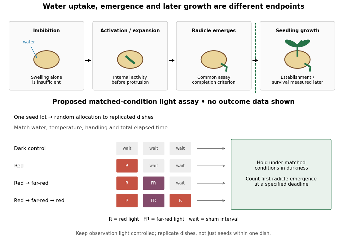
Seed germination is renewed plant embryo activity and growth. Many germination assays score completion as radicle emergence, before seedling establishment. Seed imbibition precedes that endpoint; swelling alone is insufficient.^[ref]

Water, molecular oxygen and suitable temperature support germination; light sensitivity depends on the species and seed state. Neither illumination nor one particular temperature is universally required. Seed dormancy connects germination timing to ecology by delaying seedling establishment.^[ref]

The distinction matters when comparing propagation experiments: a treatment that increases radicle emergence need not improve later seedling survival. Define the endpoint before comparing treatments, then measure the later outcome separately.

A specified test for germination, recording the endpoint, conditions and observation window. For a proposed red/far-red light test, use randomization to allocate one seed lot to darkness, red, red then far-red, and red then far-red then red. Match hydration, temperature, handling and elapsed time before counting; use sham waiting periods to equalize schedules. Use dish replication, retain the dark scientific control, and record radicle emergence using an observation procedure that does not itself provide an uncontrolled light treatment. This is a proposed design, not a claim about the 1952 paper's randomization or replication.

As an original hypothetical counting example, begin with $N=40$ seeds in one dish. Suppose 12 first meet the radicle endpoint by 24 hours, eight additional seeds by 48 hours, and four additional seeds by 72 hours. These invented event counts giveand cumulative sample proportions $\hat{G}(24)=0.30$, $\hat{G}(48)=0.50$ and $\hat{G}(72)=0.60$. The 48-hour increment is $8/40=0.20$, not $0.50$; the latter includes earlier events. Counting the same emerged radicle again at each inspection would inflate the total. These numbers illustrate bookkeeping, not biological rates or treatment effects.

With a fixed denominator and irreversible classification of the first endpoint event, the set counted at an earlier inspection is a subset of the set counted later. Hence $0\le \hat{G}(t)\le 1$ and $\hat{G}(t)$ cannot decrease. This short proof applies to cumulative germination counts even if a later seedling dies. A count of currently surviving seedlings has a different definition and can decrease.

For treatment comparisons, the dish may be the experimental unit: seeds in the same dish share conditions. Forty seeds in one dish do not supply forty independent dish replicates. Report the sample size, replication, endpoint time and denominator; a sample proportion by a deadline measures this assay's outcome, not an unconditional fraction with seed viability.

Ivar Giaever's gap experiment used a metal–insulator–metal sandwich. His lecture describes evaporating aluminium onto glass, briefly exposing it to air to form an oxide barrier, then evaporating lead cross-strips. Cooling in liquid helium made the lead superconducting while the aluminium stayed normal in the measurements compared. A voltmeter and ammeter supplied the junction electric potential difference and electric current readouts. Thick oxides initially gave unmeasurably small electric currents; the thinner barrier made the measurement practical. Temperature comparisons and a subsequent controlled magnetic field test changed the current-voltage characteristic with the superconducting state. ^[ref]

The 1960 letter compares measurements at $4.2$ and $1.6\mathrm{K}$. An applied parallel magnetic field of $2.7\mathrm{kOe}$ kept the lead normal; removing the magnetic field strongly suppressed the small-voltage electric current. Figure 2 divides the superconducting $dI/dV$ by the normal-state slope. The letter calls its gap estimates preliminary and notes a temperature-dependent broadened peak. It also flags a limitation of interpreting tunneling directly through the density of states; the ideal NIS calculation above states additional assumptions explicitly. ^[ref]

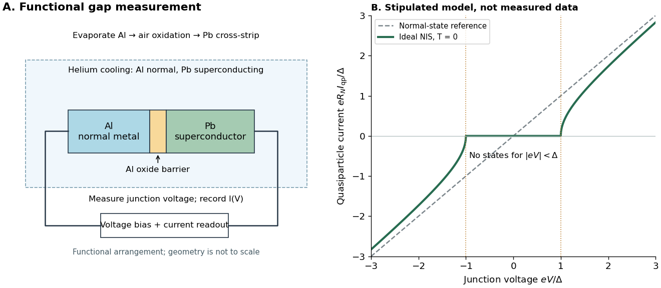
The central inference is that the barrier lets electric current interrogate available quasiparticle states. Suppression at small electric potential difference and the rise near the gap edge support a gapped spectrum; tracking the superconducting state helps distinguish that feature from an arbitrary nonlinear barrier. A leakage path through a metallic short, imperfect barrier, or an energy-dependent tunneling matrix element limits a literal density of states interpretation. The preparation and state controls therefore matter as much as seeing a nonlinear current-voltage characteristic.

William Francis Giauque's 1949 lecture, Some Consequences of Low Temperature Research in Chemical Thermodynamics, credits Peter Debye with an independent proposal. It describes gadolinium sulfate octahydrate in a jacket immersed in liquid helium, with an external solenoid. Exchange gas conducts away heat during magnetization; evacuation isolates the sample before field reduction. A liquid-nitrogen shield reduces radiative heat transfer. Its photograph identifies the 1933 apparatus operated with Duncan Peck MacDougall. An inductance bridge reads the sample's magnetic susceptibility; measuring coils remain outside the evacuated jacket in liquid helium. Increasing magnetic susceptibility indicates cooling, but converting it to temperature using Curie's law becomes approximate as that law fails.^[ref]

The measurement logic deserves a separate check. A changed inductance alone is not an absolute temperature calibration: the sample geometry, applied measuring magnetic field, and constitutive response enter the inference. A modern control would compare the susceptibility-based thermometer with an independently calibrated thermometer over their common range, check recovery after repeated sweeps, and measure subsequent warming to bound incoming heat. These are proposed controls derived from the readout principle, rather than additional procedures attributed to the 1933 experiment. The historical working salt has a richer magnetic level structure than the illustrative two-level paramagnetic cooling model.

The Euler theorem for homogeneous functions applied to an extensive quantity, together with $dE=TdS-pdV+\mu dN$ give

The Gibbs-Duhem equation constrains changes of the intensive quantities describing one uniform thermodynamic phase. For a mixture with $k$ independently specified component amounts, its molar form isHere $S$ is entropy, $V$ is volume, $T$ is temperature, $p$ is pressure, $n_i$ is the amount of substance of component $i$, and ${\mu }_i$ is its molar chemical potential. This assumes a simple compressible system whose bulk internal energy is an extensive quantity; additional work coordinates require additional terms.^[ref]

The proof exposes the source of the constraint. For internal energy $E(S,V,n_1,\dots ,n_k)$, replication of the whole thermodynamic phase by a factor $\lambda$ gives $E(\lambda S,\lambda V,\lambda n_1,\dots ,\lambda n_k)=\lambda E(S,V,n_1,\dots ,n_k)$. The Euler theorem for homogeneous functions and the fundamental differential of internal energy therefore giveTaking the differential of the first equation produces all the terms in the second, plus $SdT-Vdp+{\sum }_i{n}_{i}d{\mu }_i$. Subtraction proves the Gibbs-Duhem equation. Thus the constraint comes from two descriptions of the same state function, rather than an assumed microscopic interaction model.

At fixed temperature and pressure, divide by $n={\sum }_i{n}_i>0$ and introduce the mole fractions $x_i=n_i/n$:The chemical potentials cannot be varied independently. In a two-component mixture, put $x_A=x$ and $x_B=1-x$. Within a smooth single-thermodynamic phase region with $0<x<1$,One chemical potential fixes the other's change, but determining its absolute value still requires a reference value. This does not say ${\mu }_A={\mu }_B$: equality at phase coexistence concerns the same chemical species in different thermodynamic phases. Nor does the constraint say $dG=0$ whenever temperature and pressure are fixed; changing composition still contributes ${\sum }_i{\mu }_{i}d{n}_i$ to the Gibbs free energy.

The derivative of Gibbs energy with respect to reaction extent at fixed temperature and pressure: ${\Delta }_{r}G={\sum }_i{\nu }_i{\mu }_i$. For a reversible electrochemical cell reaction, ${\Delta }_{r}G=-nFE$.

The Gibbs free energy iswhere $H$ is enthalpy. For a closed system of fixed composition, with only pressure-volume work, spontaneous relaxation at fixed temperature and pressure cannot increase $G$; stable thermodynamic equilibrium minimizes it over the allowed states. A loaded piston can move while maintaining the imposed pressure, so the enthalpy term includes the displacement cost. Along a smooth equilibrium branch of fixed composition,Thus its temperature slope at fixed pressure is $-S$, while its pressure slope at fixed temperature is $V$. See MIT 5.60, Lecture 13, Gibbs free energy and its derivatives.

Consider two illustrative thermodynamic phases, A and B, of the same substance at one fixed pressure. Write B minus A, using quantities per mole:Treat these differences as approximately constant over a limited temperature window. ThenAt $280\mathrm{K}$, $\Delta G=+0.8\mathrm{kJ}\mathrm{mo}{\mathrm{l}}^{-1}$, so A is preferred. At $320\mathrm{K}$, $\Delta G=-0.8\mathrm{kJ}\mathrm{mo}{\mathrm{l}}^{-1}$, so B is preferred. At $300\mathrm{K}$, both have equal molar Gibbs free energy, permitting phase coexistence in this bulk model. B's greater entropy outweighs its greater enthalpy above the crossing.

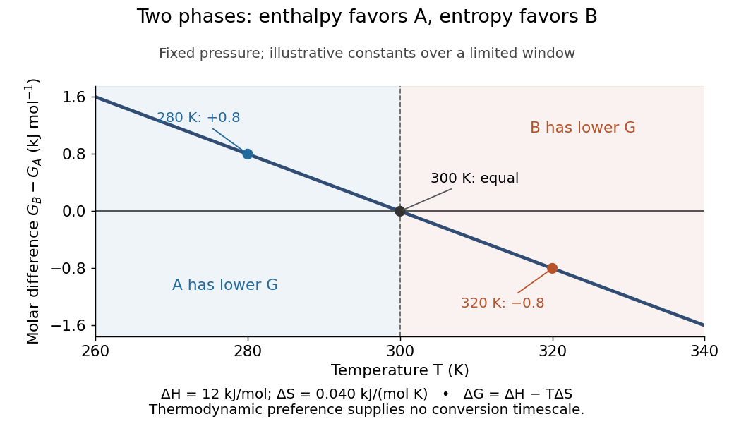
Each plotted point compares alternatives at the same temperature; moving along the curve changes the imposed temperature. The model predicts preference, not instantaneous conversion: nucleation barriers can sustain metastability. Real enthalpy and entropy differences generally vary with temperature through heat capacities, bending this line outside the approximation.

At fixed pressure, the first law of thermodynamics gives $Q=\Delta H$ under the stated work restriction, so the same thermal reservoir accounting yields $\Delta S_{\mathrm{total}}=-\Delta G/T\ge 0$. Variable composition restores ${\sum }_i{\mu }_{i}d{n}_i$ to $dG$; constrained Gibbs minimization for chemical equilibrium handles those permitted changes.

The historical foundation is Gibbs's ^[ref]. Its equations (87) and (91) introduce the combinations now called Helmholtz free energy and Gibbs free energy, connecting entropy criteria, chemical potentials and phase coexistence within one framework.

For the equation of state $V=N{k}_{B}T/p-NA(T)$, integrate $(\partial G/\partial p{)}_{T,N}=V$ along an isotherm. This gives the displayed Gibbs free energy difference. Its negative temperature derivative at fixed endpoint pressures gives $\Delta S=-N{k}_B\ln (p_1/p_0)+N{A}^{\prime }(T)(p_1-p_0)$. The physically admissible branch must retain positive volume.

For a single-phase ideal gas mixture with molar amounts $N_i$, common temperature $T$, and pressure $P$, extensivity and ideal mixing giveHere $N={\sum }_i{N}_i$, $x_i$ is the mole fraction, $\mathcal{R}$ is the molar gas constant, and $P^{\circ }$ is the standard pressure. Integrating $\partial {\mu }_i/\partial P=\mathcal{R}T/P$ and including the ideal mixing entropy proves ${\mu }_i={\mu }_i^{\circ }+\mathcal{R}T\log (x_{i}P/P^{\circ })$. Reactions can change $N$, so fractions alone do not set the extensive Gibbs free energy. Its composition Hessian is $\mathcal{R}T({\delta }_{ij}/N_i-1/N)$; it is positive semidefinite by the weighted Cauchy-Schwarz inequality.

The Gibbs free energy of mixing compares the final mixture's Gibbs free energy with that of its initially separate components at the same temperature and pressure. For an ideal solution, subtract the pure-component reference from $G={\sum }_i{n}_i{\mu }_i$:For one mole of the chosen A/B ideal solution at $300\mathrm{K}$ and $x_A=0.4$,The individual chemical potential changes are $RT\ln 0.4\approx -2.28554\mathrm{kJ}\mathrm{mo}{\mathrm{l}}^{-1}$ for A and $RT\ln 0.6\approx -1.27417\mathrm{kJ}\mathrm{mo}{\mathrm{l}}^{-1}$ for B. Weighting these by $0.4\mathrm{mol}$ and $0.6\mathrm{mol}$ reproduces the total Gibbs free energy of mixing.

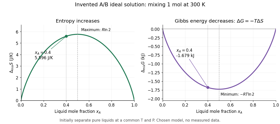
If ideality holds in a neighborhood of the specified temperature and pressure, differentiation at fixed component amounts givesThus the ideal mixing Gibbs free energy decrease comes entirely from the entropy increase; the mixing enthalpy and volume changes vanish. Ideality at a single isolated state alone does not determine temperature or pressure derivatives.^[ref]

The same formula rules out spontaneous separation into two liquid thermodynamic phases within this model. Per mole, the mixing Gibbs free energy $g_{\mathrm{mix}}=RT[x\ln x+(1-x)\ln (1-x)]$ hasAdding the pure-component reference contributions changes only a term linear in $x$. The total molar Gibbs free energy is therefore a strictly convex function: a separated pair of different compositions has a larger composition-weighted Gibbs free energy than the uniform sample with the same inventory. Such phase separation requires physics beyond this ideal solution model.

For fixed composition and pressure, $\partial (G/T)/\partial T=-H/T^2$. Applying the identity to standard reaction quantities connects equilibrium temperature dependence to reaction enthalpy.